Exploring and understanding data
Last updated on 2025-10-29 | Edit this page
Overview
Questions
- How can I do exploratory data analysis in Python?
- How do I get help when I am stuck?
- What impact does an object’s type have on what I can do with it?
- How are expressions evaluated and values assigned to variables?
Objectives
- Explore the structure and content of pandas dataframes
- Convert data types and handle missing data
- Interpret error messages and develop strategies to get help with Python
- Trace how Python assigns values to objects
The pandas DataFrame
We just spent quite a bit of time learning how to create
visualisations from the samples data, but we did not talk
much about what samples is. Let’s first load the data
again:
You may remember that we loaded the data into Python with the
pandas.read_csv function. The output of
read_csv is a data frame: a common way of
representing tabular data in a programming language. To be precise,
samples is an object of type
DataFrame. In Python, pretty much everything you work with
is an object of some type. The type function can be used to
tell you the type of any object you pass to it.
OUTPUT
pandas.core.frame.DataFrameThis output tells us that the DataFrame object type is
defined by pandas, i.e. it is a special type of object not included in
the core functionality of Python.
Exploring data in a dataframe
We encountered the plot, head and
tail methods in the previous epsiode. Dataframe objects
carry many other methods, including some that are useful when exploring
a dataset for the first time. Consider the output of
describe:
OUTPUT
              month           day 	       year       plot_id  hindfoot_length 	      weight
count  16878.000000  16878.000000  16878.000000  16878.000000     14145.000000  15186.000000
mean       6.382214     15.595805   1983.582119     11.471442        31.982114     53.216647
std        3.411215      8.428180      3.492428      6.865875        10.709841     44.265878
min        1.000000      1.000000   1977.000000      1.000000         6.000000      4.000000
25%        3.000000      9.000000   1981.000000      5.000000        21.000000     24.000000
50%        6.000000     15.000000   1983.000000     11.000000        35.000000     42.000000
75%        9.000000     23.000000   1987.000000     17.000000        37.000000     53.000000
max       12.000000     31.000000   1989.000000     24.000000        70.000000    278.000000
These summary statistics give an immediate impression of the distribution of the data. It is always worth performing an initial “sniff test” with these: if there are major issues with the data or its formatting, they may become apparent at this stage.
info provides an overview of the columns included in the
dataframe:
OUTPUT
<class 'pandas.core.frame.DataFrame'>
Index: 16878 entries, 1 to 16878
Data columns (total 12 columns):
 #   Column           Non-Null Count  Dtype
---  ------           --------------  -----
 0   month            16878 non-null  int64
 1   day              16878 non-null  int64
 2   year             16878 non-null  int64
 3   plot_id          16878 non-null  int64
 4   species_id       16521 non-null  object
 5   sex              15578 non-null  object
 6   hindfoot_length  14145 non-null  float64
 7   weight           15186 non-null  float64
 8   genus            16521 non-null  object
 9   species          16521 non-null  object
 10  taxa             16521 non-null  object
 11  plot_type        16878 non-null  object
dtypes: float64(2), int64(4), object(6)
memory usage: 1.7+ MB
We get quite a bit of useful information here too. First, we are told
that we have a DataFrame of 16878 entries, or rows, and 12
variables, or columns.
Next, we get a bit of information on each variable, including its
column title, a count of the non-null values (that is, values
that are not missing), and something called the dtype of
the column.
Data types
The dtype property of a dataframe column describes the
data type of the values stored in that column. There are three
in the example above:
-
int64: this column contains integer (whole number) values. -
object: this column contains string (non-numeric sequence of characters) values. -
float64: this column contains “floating point” values i.e. numeric values containing a decimal point.
The 64 after int and float
represents the level of precision with which the values in the column
are stored in the computer’s memory. Other types with lower levels of
precision are available for numeric values, e.g. int32 and
float16, which will take up less memory on your system but
limit the size and level of precision of the numbers they can store.
The dtype of a column is important because it determines
the kinds of operation that can be performed on the values in that
column. Let’s work with a couple of the columns independently to
demonstrate this.
The Series object
To work with a single column of a dataframe, we can refer to it by name in two different ways:
or
PYTHON
samples.species_id # this only works if there are no spaces in the column name (note the underscore used here)OUTPUT
record_id
1        NL
2        NL
3        DM
4        DM
5        DM
         ..
16874    RM
16875    RM
16876    DM
16877    DM
16878    DM
Name: species_id, Length: 16878, dtype: objectTip: use tab completion on column names
Tab completion, where you start typing the name of a variable, function, etc before hitting Tab to auto-complete the rest, also works on column names of a dataframe. Since this tab completion saves time and reduces the chance of including typos, we recommend you use it as frequently as possible.
The result of that operation is a series of data: a
one-dimensional sequence of values that all have the same
dtype (object in this case). Dataframe objects
are collections of the series “glued together” with a shared
index: the column of unique identifiers we associate with each
row. record_id is the index of the series summarised above;
the values carried by the series are NL, DM,
AH, etc (short species identification codes).
If we choose a different column of the dataframe, we get another series with a different data type:
OUTPUT
record_id
1         NaN
2         NaN
3         NaN
4         NaN
5         NaN
         ...
16874    15.0
16875     9.0
16876    31.0
16877    50.0
16878    42.0
Name: weight, Length: 16878, dtype: float64
The data type of the series influences the things that can be done
with/to it. For example, sorting works differently for these two series,
with the numeric values in the weight series sorted from
largest to smallest and the character strings in species_id
sorted alphabetically:
OUTPUT
record_id
9790     4.0
5346     4.0
4052     4.0
9853     4.0
7084     4.0
        ...
16772    NaN
16777    NaN
16808    NaN
16846    NaN
16860    NaN
Name: weight, Length: 16878, dtype: float64OUTPUT
record_id
12345     AB
9861      AB
10970     AB
10963     AB
5759      AB
        ...
16453    NaN
16454    NaN
16488    NaN
16489    NaN
16539    NaN
Name: species_id, Length: 16878, dtype: object
This pattern of behaviour, where the type of an object determines
what can be done with it and influences how it is done, is a defining
characteristic of Python. As you gain more experience with the language,
you will become more familiar with this way of working with data. For
now, as you begin on your learning journey with the language, we
recommend using the type function frequently to make sure
that you know what kind of data/object you are working with, and do not
be afraid to ask for help whenever you are unsure or encounter a
problem.
Aside: Getting Help
You may have already encountered several errors while following the lesson and this is a good time to take a step back and discuss good strategies to get help when something goes wrong.
The built-in help function
Use help to view documentation for an object or
function. For example, if you want to see documentation for the
round function:
OUTPUT
Help on built-in function round in module builtins:

round(number, ndigits=None)
    Round a number to a given precision in decimal digits.

    The return value is an integer if ndigits is omitted or None.  Otherwise
    the return value has the same type as the number.  ndigits may be negative.
The Jupyter Notebook has two ways to get help.
If you are working in Jupyter (Notebook or Lab), the platform offers some additional ways to see documentation/get help:
- Option 1: Type the function name in a cell with a question mark
after it, e.g.
round?. Then run the cell. - Option 2: (Not available on all systems) Place the cursor near where
the function is invoked in a cell (i.e., the function name or its
parameters),
- Hold down Shift, and press Tab.
- Do this several times to expand the information returned.
Understanding error messages
The error messages returned when something goes wrong can be (very)
long but contain information about the problem, which can be very useful
once you know how to interpret it. For example, you might receive a
SyntaxError if you mistyped a line and the resulting code
was invalid:
ERROR
  Cell In[129], line 1
    name = 'Feng
           ^
SyntaxError: unterminated string literal (detected at line 1)
There are three parts to this error message:
ERROR
Cell In[129], line 1This tells us where the error occured. This is of limited help in
Jupyter, since we know that the error is in the cell we just ran
(Cell In[129]), but the line number can be helpful
especially when the cell is quite long. But when running a larger
program written in Python, perhaps built up from multiple individual
scripts, this can be more useful, e.g.
ERROR
data_visualisation.py, line 42Next, we see a copy of the line where the error was encountered, often annotated with an arrow pointing out exactly where Python thinks the problem is:
ERROR
    name = 'Feng
           ^
Python is not exactly right in this case: from context you might be able to guess that the issue is really the lack of a closing quotation mark at the end of the line. But an arrow pointing to the opening quotation mark can give us a push in the right direction. Sometimes Python gets these annotations exactly right. Occasionally, it gets them completely wrong. In the vast majority of cases they are at least somewhat helpful.
Finally, we get the error message itself:
ERROR
SyntaxError: unterminated string literal (detected at line 1)This always begins with a statement of the type of error
encountered: in this case, a SyntaxError. That provides a
broad categorisation for what went wrong. The rest of the message is a
description of exactly what the problem was from Python’s perspective.
Error messages can be loaded with jargon and quite difficult to
understand when you are first starting out. In this example,
unterminated string literal is a technical way of saying
“you opened some quotes, which I think means you were trying to define a
string value, but the quotes did not get closed before the end of the
line.”
It is normal not to understand exactly what these error messages mean the first time you encounter them. Since programming involves making lots of mistakes (for everyone!), you will start to become familiar with many of them over time. As you continue learning, we recommend that you ask others for help: more experienced programmers have made all of these mistakes before you and will probably be better at spotting what has gone wrong. (More on asking for help below.)
Error output can get really long!
Especially when using functions from libraries you have imported into your program, the middle part of the error message (the traceback) can get rather long. For example, what happens if we try to access a column that does not exist in our dataframe?
ERROR
---------------------------------------------------------------------------
KeyError                                  Traceback (most recent call last)
File ~/miniforge3/envs/carpentries/lib/python3.11/site-packages/pandas/core/indexes/base.py:3812, in Index.get_loc(self, key)
   3811 try:
-> 3812     return self._engine.get_loc(casted_key)
   3813 except KeyError as err:

File pandas/_libs/index.pyx:167, in pandas._libs.index.IndexEngine.get_loc()

File pandas/_libs/index.pyx:196, in pandas._libs.index.IndexEngine.get_loc()

File pandas/_libs/hashtable_class_helper.pxi:7088, in pandas._libs.hashtable.PyObjectHashTable.get_item()

File pandas/_libs/hashtable_class_helper.pxi:7096, in pandas._libs.hashtable.PyObjectHashTable.get_item()

KeyError: 'wegiht'

The above exception was the direct cause of the following exception:

KeyError                                  Traceback (most recent call last)
Cell In[131], line 1
----> 1 samples['wegiht']

File ~/miniforge3/envs/carpentries/lib/python3.11/site-packages/pandas/core/frame.py:4107, in DataFrame.__getitem__(self, key)
   4105 if self.columns.nlevels > 1:
   4106     return self._getitem_multilevel(key)
-> 4107 indexer = self.columns.get_loc(key)
   4108 if is_integer(indexer):
   4109     indexer = [indexer]

File ~/miniforge3/envs/carpentries/lib/python3.11/site-packages/pandas/core/indexes/base.py:3819, in Index.get_loc(self, key)
   3814     if isinstance(casted_key, slice) or (
   3815         isinstance(casted_key, abc.Iterable)
   3816         and any(isinstance(x, slice) for x in casted_key)
   3817     ):
   3818         raise InvalidIndexError(key)
-> 3819     raise KeyError(key) from err
   3820 except TypeError:
   3821     # If we have a listlike key, _check_indexing_error will raise
   3822     #  InvalidIndexError. Otherwise we fall through and re-raise
   3823     #  the TypeError.
   3824     self._check_indexing_error(key)

KeyError: 'wegiht'
(This is still relatively short compared to some errors messages we have seen!)
When you encounter a long error like this one, do not panic! Our advice is to focus on the first couple of lines and the last couple of lines. Everything in the middle (as the name traceback suggests) is retracing steps through the program, identifying where problems were encountered along the way. That information is only really useful to somebody interested in the inner workings of the pandas library, which is well beyond the scope of this lesson! If we ignore everything in the middle, the parts of the error message we want to focus on are:
ERROR
---------------------------------------------------------------------------
KeyError                                  Traceback (most recent call last)

[... skipping these parts ...]

KeyError: 'wegiht'
This tells us that the problem is the “key”: the value we used to lookup the column in the dataframe. Hopefully, the repetition of the value we provided would be enough to help us realise our mistake.
Other ways to get help
There are several other ways that people often get help when they are stuck with their Python code.
- Search the internet: paste the last line of your error message or
the word “python” and a short description of what you want to do into
your favourite search engine and you will usually find several examples
where other people have encountered the same problem and came looking
for help.
- StackOverflow can be particularly helpful for this: answers to questions are presented as a ranked thread ordered according to how useful other users found them to be.
- Take care: copying and pasting code written by somebody else is risky unless you understand exactly what it is doing!
- ask somebody “in the real world”. If you have a colleague or friend with more expertise in Python than you have, show them the problem you are having and ask them for help.
- Sometimes, the act of articulating your question can help you to identify what is going wrong. This is known as “rubber duck debugging” among programmers.
Generative AI
It is increasingly common for people to use generative AI chatbots such as ChatGPT to get help while coding. You will probably receive some useful guidance by presenting your error message to the chatbot and asking it what went wrong. However, the way this help is provided by the chatbot is different. Answers on StackOverflow have (probably) been given by a human as a direct response to the question asked. But generative AI chatbots, which are based on an advanced statistical model, respond by generating the most likely sequence of text that would follow the prompt they are given.
While responses from generative AI tools can often be helpful, they are not always reliable. These tools sometimes generate plausible but incorrect or misleading information, so (just as with an answer found on the internet) it is essential to verify their accuracy. You need the knowledge and skills to be able to understand these responses, to judge whether or not they are accurate, and to fix any errors in the code it offers you.
In addition to asking for help, programmers can use generative AI tools to generate code from scratch; extend, improve and reorganise existing code; translate code between programming languages; figure out what terms to use in a search of the internet; and more. However, there are drawbacks that you should be aware of.
The models used by these tools have been “trained” on very large volumes of data, much of it taken from the internet, and the responses they produce reflect that training data, and may recapitulate its inaccuracies or biases. The environmental costs (energy and water use) of LLMs are a lot higher than other technologies, both during development (known as training) and when an individual user uses one (also called inference). For more information see the AI Environmental Impact Primer developed by researchers at HuggingFace, an AI hosting platform. Concerns also exist about the way the data for this training was obtained, with questions raised about whether the people developing the LLMs had permission to use it. Other ethical concerns have also been raised, such as reports that workers were exploited during the training process.
We recommend that you avoid getting help from generative AI during the workshop for several reasons:
- For most problems you will encounter at this stage, help and answers can be found among the first results returned by searching the internet.
- The foundational knowledge and skills you will learn in this lesson by writing and fixing your own programs are essential to be able to evaluate the correctness and safety of any code you receive from online help or a generative AI chatbot. If you choose to use these tools in the future, the expertise you gain from learning and practising these fundamentals on your own will help you use them more effectively.
- As you start out with programming, the mistakes you make will be the kinds that have also been made – and overcome! – by everybody else who learned to program before you. Since these mistakes and the questions you are likely to have at this stage are common, they are also better represented than other, more specialised problems and tasks in the data that was used to train generative AI tools. This means that a generative AI chatbot is more likely to produce accurate responses to questions that novices ask, which could give you a false impression of how reliable they will be when you are ready to do things that are more advanced.
Data input within Python
Although it is more common (and faster) to input data in another format e.g. a spreadsheet and read it in, Series and DataFrame objects can be created directly within Python. Before we can make a new Series, we need to learn about another type of data in Python: the list.
Lists
Lists are one of the standard data structures built into
Python. A data structure is an object that contains more than one piece
of information. (DataFrames and Series are also data structures.) The
list is designed to contain multiple values in an ordered sequence: they
are a great choice if you want to build up and modify a collection of
values over time and/or handle each of those values one at a time. We
can create a new list in Python by capturing the values we want it to
store inside square brackets []:
OUTPUT
[2020, 2025, 2010]New values can be added to the end of a list with the
append method:
OUTPUT
[2020, 2025, 2010, 2015]Exploring list methods
The append method allows us to add a value to the end of
a list but how could we insert a new value into a given position
instead? Applying what you have learned about how to find out the
methods that an object has, can you figure out how to place the value
2019 into the third position in years_list
(shifting the values after it up one more position)? Recall that the
indexing used to specify positions in a sequence begins at 0 in
Python.
Using tab completion, the help function, or looking up
the documentation online, we can discover the insert method
and learn how it works. insert takes two arguments: the
position for the new list entry and the value to be placed in that
position:
OUTPUT
[2020, 2025, 2019, 2010, 2015]Among many other methods is sort, which can be used to
sort the values in the list:
OUTPUT
[2010, 2015, 2019, 2020, 2025]The easiest way to create a new Series is with a list:
OUTPUT
0    2010
1    2015
2    2019
3    2020
4    2025
dtype: int64
With the data in a Series, we can no longer do some of the things we were able to do with the list, such as adding new values. But we do gain access to some new possibilities, which can be very helpful. For example, if we wanted to increase all of the values by 1000, this would be easy with a Series but more complicated with a list:
OUTPUT
0    3010
1    3015
2    3019
3    3020
4    3025
dtype: int64ERROR
---------------------------------------------------------------------------
TypeError                                 Traceback (most recent call last)
Cell In[126], line 1
----> 1 years_list + 1000

TypeError: can only concatenate list (not "int") to list
This illustrates an important principle of Python: different data structures are suitable for different “modes” of working with data. It can be helpful to work with a list when building up an initial set of data from scratch, but when you are ready to begin operating on that dataset as a whole (performing calculations with it, visualising it, etc), you will be rewarded for switching to a more specialised datatype like a Series or DataFrame from pandas.
Unexpected data types
Operations like the addition of 1000 we performed on
years_series work because pandas knows how to add a number
to the integer values in the series. That behaviour is determind by the
dtype of the series, which makes that dtype
really important for how you want to work with your data. Let’s explore
how the dtype is chosen. Returning to the
years_series object we created above:
OUTPUT
0    2010
1    2015
2    2019
3    2020
4    2025
dtype: int64
The dtype: int64 was determined automatically based on
the values passed in. But what if the values provided are of several
different types?
OUTPUT
0    2.0
1    3.0
2    5.5
3    6.0
4    8.0
dtype: float64
Pandas assigns a dtype that allows it to account for all
of the values it is given, converting some values to another
dtype if needed, in a process called coercion. In
the case above, all of the integer values were coerced to floating point
numbers to account for the 5.5.
In practice, it is much more common to read data from elsewhere
(e.g. with read_csv) than to enter it manually within
Python. When reading data from a file, pandas tries to guess the
appropriate dtype to assign to each column (series) of the
dataframe. This is usually very helpful but the process is sensitive to
inconsistencies and data entry errors in the input: a stray character in
one cell can cause an entire column to be coerced to a different
dtype than you might have wanted.
For example, if the raw data includes a symbol added by a typo
mistake (= instead of -):
name,latitude,longitude
Superior,47.7,-87.5
Victoria,-1.0,33.0
Tanganyika,=6.0,29.3
We see a non-numeric dtype for the latitude column
(object) when we load the data into a dataframe.
OUTPUT
<class 'pandas.core.frame.DataFrame'>
RangeIndex: 3 entries, 0 to 2
Data columns (total 3 columns):
 #   Column     Non-Null Count  Dtype
---  ------     --------------  -----
 0   name       3 non-null      object
 1   latitude   3 non-null      object
 2   longitude  3 non-null      float64
dtypes: float64(1), object(2)
memory usage: 200.0+ bytes
It is a good idea to run the info method on a new
dataframe after you have loaded data for the first time: if one or more
of the columns has a different dtype than you expected,
this may be a signal that you need to clean up the raw data.
Recasting
A column can be manually coerced (or recast) into a
different dtype, provided that pandas knows how to handle
that conversion. For example, the integer values in the
plot_id column of our dataframe can be converted to
floating point numbers:
OUTPUT
record_id
record_id
1         2.0
2         3.0
3         2.0
4         7.0
5         3.0
         ...
16874    16.0
16875     5.0
16876     4.0
16877    11.0
16878     8.0
Name: plot_id, Length: 16878, dtype: float64
But the string values of species_id cannot be converted
to numeric data:
ERROR
---------------------------------------------------------------------------
ValueError                                Traceback (most recent call last)
Cell In[101], line 1
----> 1 samples.species_id = samples.species_id.astype('int64')

File ~/miniforge3/envs/carpentries/lib/python3.11/site-packages/pandas/core/generic.py:6662, in NDFrame.astype(self, dtype, copy, errors)
   6656     results = [
   6657         ser.astype(dtype, copy=copy, errors=errors) for _, ser in self.items()
   6658     ]
   6660 else:
   6661     # else, only a single dtype is given
-> 6662     new_data = self._mgr.astype(dtype=dtype, copy=copy, errors=errors)
   6663     res = self._constructor_from_mgr(new_data, axes=new_data.axes)
   6664     return res.__finalize__(self, method="astype")

[... a lot more lines of traceback ...]

File ~/miniforge3/envs/carpentries/lib/python3.11/site-packages/pandas/core/dtypes/astype.py:133, in _astype_nansafe(arr, dtype, copy, skipna)
    129     raise ValueError(msg)
    131 if copy or arr.dtype == object or dtype == object:
    132     # Explicit copy, or required since NumPy can't view from / to object.
--> 133     return arr.astype(dtype, copy=True)
    135 return arr.astype(dtype, copy=copy)

ValueError: invalid literal for int() with base 10: 'NL'Changing Types
- Convert the values in the column
plot_idback to integers. - Now try converting
weightto an integer. What goes wrong here? What is pandas telling you? We will talk about some solutions to this later.
OUTPUT
record_id
1         2
2         3
3         2
4         7
5         3
         ..
16874    16
16875     5
16876     4
16877    11
16878     8
Name: plot_id, Length: 16878, dtype: int64ERROR
pandas.errors.IntCastingNaNError: Cannot convert non-finite values (NA or inf) to integerPandas cannot convert types from float to int if the column contains missing values.
Missing Data
In addition to data entry errors, it is common to encounter missing values in large volumns of data. A value may be missing because it was not possible to make a complete observation, because data was lost, or for any number of other reasons. It is important to consider missing values while processing data because they can influence downstream analysis – that is, data analysis that will be done later – in unwanted ways when not handled correctly.
Depending on the dtype of the column/series, missing
values may appear as NaN (“Not a Number”),
NA, <NA>, or NaT (“Not
a Time”). You may have noticed some during our initial exploration
of the dataframe. (Note the NaN values in the first five
rows of the weight column below.)
OUTPUT
           month  day  year  plot_id  species_id  sex  hindfoot_length  weight      genus   species    taxa                 plot_type
record_id
1              7   16  1977        2          NL    M             32.0     NaN    Neotoma  albigula  Rodent                   Control
2              7   16  1977        3          NL    M             33.0     NaN    Neotoma  albigula  Rodent  Long-term Krat Exclosure
3              7   16  1977        2          DM    F             37.0     NaN  Dipodomys  merriami  Rodent                   Control
4              7   16  1977        7          DM    M             36.0     NaN  Dipodomys  merriami  Rodent          Rodent Exclosure
5              7   16  1977        3          DM    M             35.0     NaN  Dipodomys  merriami  Rodent  Long-term Krat Exclosure
The output of the info method includes a count of the
non-null values – that is, the values that are not
missing – for each column:
OUTPUT
<class 'pandas.core.frame.DataFrame'>
Index: 16878 entries, 1 to 16878
Data columns (total 12 columns):
 #   Column           Non-Null Count  Dtype
---  ------           --------------  -----
 0   month            16878 non-null  int64
 1   day              16878 non-null  int64
 2   year             16878 non-null  int64
 3   plot_id          16878 non-null  int64
 4   species_id       16521 non-null  object
 5   sex              15578 non-null  object
 6   hindfoot_length  14145 non-null  float64
 7   weight           15186 non-null  float64
 8   genus            16521 non-null  object
 9   species          16521 non-null  object
 10  taxa             16521 non-null  object
 11  plot_type        16878 non-null  object
dtypes: float64(2), int64(4), object(6)
memory usage: 1.7+ MB
From this output we can tell that almost 1700 weight measurements and more than 2700 hindfoot length measurements are missing. Many of the other columns also have missing values.
The ouput above demonstrates that pandas can distinguish these
NaN values from the actual data and indeed they will be
ignored for some tasks, such as calculation of the summary statistics
provided by describe.
OUTPUT
              month           day 	       year       plot_id  hindfoot_length 	      weight
count  16878.000000  16878.000000  16878.000000  16878.000000     14145.000000  15186.000000
mean       6.382214     15.595805   1983.582119     11.471442        31.982114     53.216647
std        3.411215      8.428180      3.492428      6.865875        10.709841     44.265878
min        1.000000      1.000000   1977.000000      1.000000         6.000000      4.000000
25%        3.000000      9.000000   1981.000000      5.000000        21.000000     24.000000
50%        6.000000     15.000000   1983.000000     11.000000        35.000000     42.000000
75%        9.000000     23.000000   1987.000000     17.000000        37.000000     53.000000
max       12.000000     31.000000   1989.000000     24.000000        70.000000    278.000000
In some circumstances, like the recasting we attempted in the previous exercise, the missing values can cause trouble. It is up to us to decide how best to handle those missing values. We could remove the rows containing missing data, accepting the loss of all data for that observation:
OUTPUT
           month  day  year  plot_id species_id sex  hindfoot_length  weight      genus   species    taxa                 plot_type
record_id
63             8   19  1977        3         DM   M             35.0    40.0  Dipodomys  merriami  Rodent  Long-term Krat Exclosure
64             8   19  1977        7         DM   M             37.0    48.0  Dipodomys  merriami  Rodent          Rodent Exclosure
65             8   19  1977        4         DM   F             34.0    29.0  Dipodomys  merriami  Rodent                   Control
66             8   19  1977        4         DM   F             35.0    46.0  Dipodomys  merriami  Rodent                   Control
67             8   19  1977        7         DM   M             35.0    36.0  Dipodomys  merriami  Rodent          Rodent Exclosure
But we should take note that this removes more than 3000 rows from the dataframe!
OUTPUT
16878OUTPUT
13773Instead, we could fill all of the missing values with
something else. For example, let’s make a copy of the
samples dataframe then populate the missing values in the
weight column of that copy with the mean of all the
non-missing weights. There are a few parts to that operation, which are
tackled one at a time below.
PYTHON
mean_weight = samples['weight'].mean() # the 'mean' method calculates the mean of the non-null values in the column
df1 = samples.copy() # making a copy to work with so that we do not edit our original data
df1['weight'] = df1['weight'].fillna(mean_weight) # the 'fillna' method fills all missing values with the provided value
df1.head()
OUTPUT
           month  day  year  plot_id species_id sex  hindfoot_length     weight      genus   species    taxa                 plot_type
record_id
1              7   16  1977        2         NL   M             32.0  53.216647    Neotoma  albigula  Rodent                   Control
2              7   16  1977        3         NL   M             33.0  53.216647    Neotoma  albigula  Rodent  Long-term Krat Exclosure
3              7   16  1977        2         DM   F             37.0  53.216647  Dipodomys  merriami  Rodent                   Control
4              7   16  1977        7         DM   M             36.0  53.216647  Dipodomys  merriami  Rodent          Rodent Exclosure
5              7   16  1977        3         DM   M             35.0  53.216647  Dipodomys  merriami  Rodent  Long-term Krat Exclosure
The choice to fill in these missing values rather than removing the rows that contain them can have implications for the result of your analysis. It is important to consider your approach carefully. Think about how the data will be used and how these values will impact the scientific conclusions made from the analysis. pandas gives us all of the tools that we need to account for these issues. But we need to be cautious about how the decisions that we make impact scientific results.
Assignment, evaluation, and mutability
Stepping away from dataframes for a moment, the time has come to explore the behaviour of Python a little more.
Understanding what’s going on here will help you avoid a lot of
confusion when working in Python. When we assign something to a
variable, the first thing that happens is the righthand side gets
evaluated. So when we first ran the line y = x*3,
x*3 first gets evaluated to the value of 6, and this gets
assigned to y. The variables x and
y are independent objects, so when we change the value of
x to 10, y is unaffected. This behaviour may
be different to what you are used to, e.g. from experience working with
data in spreadsheets where cells can be linked such that modifying the
value in one cell triggers changes in others.
Multiple evaluations can take place in a single line of Python code and learning to trace the order and impact of these evaluations is a key skill.
OUTPUT
1.0In the example above, x/y is evaluated first before the
result is subtracted from 3 and the final calculated value is assigned
to z. (The brackets () are not needed in the
calculation above but are included to make the order of evaluation
clearer.) Python makes each evaluation as it needs to in order to
proceed with the next, before assigning the final result to the variable
on the lefthand side of the = operator.
This means that we could have filled the missing values in the weight column of our dataframe copy in a single line:
First, the mean weight is calculated
(df1['weight'].mean() is evaluated). Then the result of
that evaluation is passed into fillna and the result of the
filling operation
(df1['weight'].fillna(<RESULT OF PREVIOUS>)) is
assigned to df1['weight'].
Variable naming
You are going to name a lot of variables in Python! There are some rules you have to stick to when doing so, as well as recommendations that will make your life easier.
- Make names clear without being too long
-
wkgis probably too short. -
weight_in_kilogramsis probably too long. -
weight_kgis good.
-
- Names cannot begin with a number.
- Names cannot contain spaces; use underscores instead.
- Names are case sensitive:
weight_kgis a different name fromWeight_kg. Avoid uppercase characters at the beginning of variable names. - Names cannot contain most non-letter characters:
+&-/*.etc. - Two common formats of variable name are
snake_caseandcamelCase. A third “case” of naming convention,kebab-case, is not allowed in Python (see the rule above). - Aim to be consistent in how you name things within your projects. It is easier to follow an established style guide, such as Google’s, than to come up with your own.
Exercise; good variable names
Identify at least one good variable name and at least one variable name that could be improved in this episode. Refer to the rules and recommendations listed above to suggest how these variable names could be better.
mean_weight and samples are examples of
reasonably good variable names: they are relatively short yet
descriptive.
df2 is not descriptive enough and could be potentially
confusing if encountered by somebody else/ourselves in a few weeks’
time. The name could be improved by making it more descriptive,
e.g. samples_duplicate.
Mutability
Why did we need to use the copy method to duplicate the
dataframe above if variables are not linked to each other? Why not
assign a new variable with the value of the existing dataframe
object?
This gets to mutablity: a feature of Python that has caused headaches for many novices in the past! In the interests of memory management, Python avoids making copies of objects unless it has to. Some types of objects are immutable, meaning that their value cannot be modified once set. Immutable object types we have already encountered include strings, integers, and floats. If we want to adjust the value of an integer variable, we must explicitly overwrite it.
Other types of object are mutable, meaning that their value
can be changed “in-place” without needing to be explictly overwritten.
This includes lists and pandas DataFrame
objects, which can be reordered etc. after they are
created.
When a new variable is assigned the value of an existing immutable object, Python duplicates the value and assigns it to the new variable.
a = 3.5 # new float object, called "a"
b = a   # another new float object, called "b", which also has the value 3.5
When a new variable is assigned the value of an existing mutable object, Python makes a new “pointer” towards the value of the existing object instead of duplicating it.
some_species = ['NL', 'DM', 'PF', 'PE', 'DS'] # new list object, called "some_species"
some_more_species = some_species # another name for the same list object
This can have unintended consequences and lead to much confusion!
some_more_species[2] = 'CV'
some_species
OUTPUT
['NL', 'DM', 'CV', 'PE', 'DS']As you can see here, the “PV” value was replaced by “CV” in both
lists, even if we didn’t intend to make the change in the
some_species list.
This takes practice and time to get used to. The key thing to
remember is that you should use the copy method to
make a copy of your dataframes to avoid accidentally modifying
the data in the original.
Groups in Pandas
We often want to calculate summary statistics grouped by subsets or attributes within fields of our data. For example, we might want to calculate the average weight of all individuals per site.
We can calculate basic statistics for all records in a single column using the syntax below:
gives output
PYTHON
count    15186.000000
mean        53.216647
std         44.265878
min          4.000000
25%         24.000000
50%         42.000000
75%         53.000000
max        278.000000
Name: weight, dtype: float64
We can also extract one specific metric if we wish:
PYTHON
samples['weight'].min()
samples['weight'].max()
samples['weight'].mean()
samples['weight'].std()
samples['weight'].count()
But if we want to summarize by one or more variables, for example
sex, we can use Pandas’ .groupby method.
Once we’ve created a groupby DataFrame, we can quickly calculate summary
statistics by a group of our choice.
The pandas function describe will
return descriptive stats including: mean, median, max, min, std and
count for a particular column in the data. Pandas’ describe
function will only return summary values for columns containing numeric
data.
PYTHON
# Summary statistics for all numeric columns by sex
grouped_data.describe()
# Provide the mean for each numeric column by sex
grouped_data.mean(numeric_only=True)
OUTPUT
       record_id     month        day         year    plot_id  \
sex
F    8371.632960  6.475266  15.411998  1983.520361  11.418147
M    8553.106416  6.306295  15.763317  1983.679177  11.248305

     hindfoot_length     weight
sex
F           31.83258  53.114471
M           32.13352  53.164464
The groupby command is powerful in that it allows us to
quickly generate summary stats.
Challenge - Summary Data
- How many recorded individuals are female
Fand how many maleM? - What happens when you group by two columns using the following syntax and then calculate mean values?
grouped_data2 = samples.groupby(['plot_id', 'sex'])grouped_data2.mean(numeric_only=True)
- Summarize weight values for each site in your data. HINT: you can
use the following syntax to only create summary statistics for one
column in your data.
by_site['weight'].describe()
- The first column of output from
grouped_data.describe()(count) tells us that the data contains 15690 records for female individuals and 17348 records for male individuals.- Note that these two numbers do not sum to 35549, the total number of
rows we know to be in the
samplesDataFrame. Why do you think some records were excluded from the grouping?
- Note that these two numbers do not sum to 35549, the total number of
rows we know to be in the
- Calling the
mean()method on data grouped by these two columns calculates and returns the mean value for each combination of plot and sex.- Note that the mean is not meaningful for some variables, e.g. day,
month, and year. You can specify particular columns and particular
summary statistics using the
agg()method (short for aggregate), e.g. to obtain the last survey year, median foot-length and mean weight for each plot/sex combination:
- Note that the mean is not meaningful for some variables, e.g. day,
month, and year. You can specify particular columns and particular
summary statistics using the
PYTHON
samples.groupby(['plot_id', 'sex']).agg({"year": 'max',
                                           "hindfoot_length": 'median',
                                           "weight": 'mean'})
samples.groupby(['plot_id'])['weight'].describe()
OUTPUT
          count       mean        std  min   25%   50%     75%    max
plot_id
1         909.0  65.974697  45.807013  4.0  39.0  46.0   99.00  223.0
2         962.0  59.911642  50.234865  5.0  31.0  44.0   55.00  278.0
3         641.0  38.338534  50.623079  4.0  11.0  20.0   34.00  250.0
4         828.0  62.647343  41.208190  4.0  37.0  45.0  102.00  200.0
5         788.0  47.864213  36.739691  5.0  28.0  42.0   50.00  248.0
6         686.0  49.180758  36.620356  5.0  25.0  42.0   52.00  243.0
7         257.0  25.101167  31.649778  4.0  11.0  19.0   24.00  235.0
8         736.0  64.593750  43.420011  5.0  39.0  48.0  102.25  178.0
9         893.0  65.346025  41.928699  6.0  40.0  48.0   99.00  275.0
10        159.0  21.188679  25.744403  4.0  10.0  12.0   24.50  237.0
11        905.0  50.260773  37.034074  5.0  29.0  42.0   49.00  212.0
12       1086.0  55.978821  45.675559  7.0  31.0  44.0   53.00  264.0
13        647.0  56.316847  42.464628  5.0  30.5  44.0   54.00  241.0
14        798.0  52.909774  33.993126  5.0  38.0  45.0   51.00  216.0
15        357.0  35.011204  47.396960  4.0  10.0  19.0   33.00  259.0
16        232.0  26.185345  22.040403  4.0  11.0  20.0   40.00  158.0
17        788.0  59.426396  44.751988  4.0  30.0  45.0   61.25  216.0
18        690.0  56.000000  44.368296  5.0  29.0  42.0   53.00  256.0
19        369.0  19.059621  15.320905  4.0   9.0  15.0   23.00  139.0
20        662.0  65.531722  53.234713  6.0  30.0  44.0  110.75  223.0
21        342.0  24.964912  32.230001  4.0   8.0  12.0   27.00  190.0
22        611.0  70.163666  45.955603  5.0  37.0  48.0  118.00  212.0
23        209.0  21.502392  19.647158  4.0  10.0  16.0   24.00  131.0
24 631.0 50.123613 47.017531 4.0 23.0 40.0 47.00 251.0Quick & Easy Plotting Data Using Pandas
We can plot our summary stats using Pandas, too.
We can also look at how many animals were captured in each site:
PYTHON
total_count = samples.groupby('plot_id')['record_id'].nunique()
# Let's plot that too
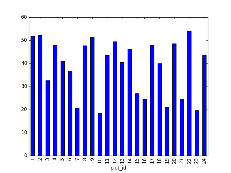
total_count.plot(kind='bar')Challenge - Plots
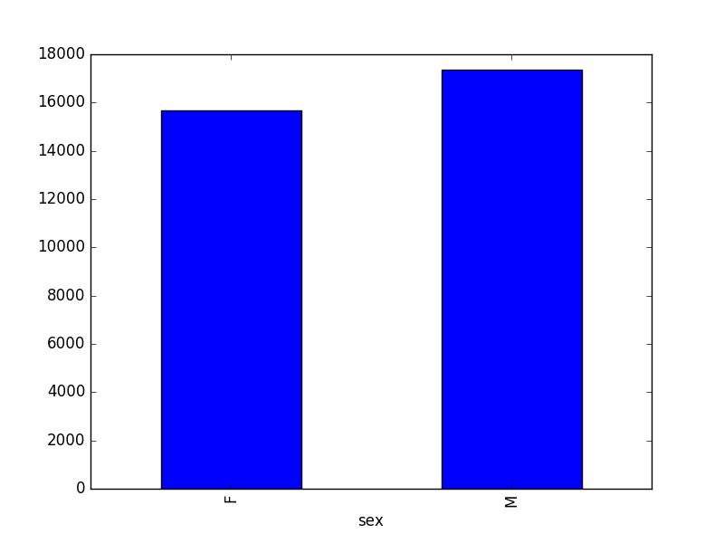
- Create a plot of average weight across all species per site.
- Create a plot of total males versus total females for the entire dataset.
samples.groupby('plot_id')["weight"].mean().plot(kind='bar')
samples.groupby('sex')["record_id"].count().plot(kind='bar')
- pandas DataFrames carry many methods that can help you explore the properties and distribution of data.
- Using the
helpfunction, reading error messages, and asking for help are all good strategies when things go wrong. - The type of an object determines what kinds of operations you can perform on and with it.
- Python evaluates expressions in a line one by one before assigning the final result to a variable.