Map 1: Campus Overview

Wide view of campus featuring bathymetry, topography, hillshade, and campus infrastructure

Rendered Map Plate

Map 1: Wide campus overview showing topography, bathymetry, bikeways, and buildings

---

Technical Summary

• Objective: Produce a broad overview plate of the UCSB campus combining elevation, ocean bathymetry, hillshading, bike path networks, and building footprints.
• Key Packages: terra, sf, tidyverse, scales
• Data Sources:
  • Campus DEM raster (source_data/campus_DEM.tif)
  • Coastal bathymetry raster (source_data/SB_bath.tif / HenleyGateEllwoodBeach.tif)
  • Campus hillshade (source_data/campus_hillshade.tif)
  • Campus buildings footprint shapefile (source_data/campus_buildings/Campus_Buildings.shp)
  • Isla Vista building footprints (source_data/iv_buildings/iv_buildings/CA_Structures_ExportFeatures.shp)
  • Bike path centerlines (source_data/icm_bikes/bike_paths/bikelanescollapsedv8.shp)
  • Modern NCOS multi-use trails (source_data/ncos_trails/ncos_multiuse_trails.geojson)
  • Lagoon & shorebird foraging habitat (source_data/NCOS_Shorebird_Foraging_Habitat/)
• Aspect Ratio: 16 inches wide x 9 inches tall (16x9).

---

Step-by-Step Cartographic Workflow & Intermediate Outputs

The generation script scripts/map_01.r iteratively layers vector features, resolves coordinate system mismatches, harmonizes disparate raster extents, and blends translucent hillshades. Below is the step-by-step breakdown:

Step 1: Initial Vector Layer Ingestion & Overlay Test

The script begins by loading the infrastructure vector layers (st_read) for campus buildings, Isla Vista structures, bike lanes, and shorebird foraging habitats. An initial unstyled ggplot checks geometry alignment.

# Initial vector load and plot check
buildings <- st_read("source_data/campus_buildings/Campus_Buildings.shp")
iv_buildings <- st_read("source_data/iv_buildings/iv_buildings/CA_Structures_ExportFeatures.shp")
bikeways <- st_read("source_data/icm_bikes/bike_paths/bikelanescollapsedv8.shp")
habitat <- st_read("source_data/NCOS_Shorebird_Foraging_Habitat/NCOS_Shorebird_Foraging_Habitat.shp")
ncos_trails <- st_read("source_data/ncos_trails/ncos_multiuse_trails.geojson")

ggplot() +
  geom_sf(data=habitat) +
  geom_sf(data=buildings) +
  geom_sf(data=iv_buildings) +
  geom_sf(data=bikeways) +
  geom_sf(data=ncos_trails) +
  coord_sf()

Intermediate Output 1.1: Raw unstyled vector layer overlays

Step 2: Applying Atlas Minimalist Theme & Color Differentiation

To eliminate clutter, a clean custom theme (my_theme) strips background fills and coordinate tick labels, leaving a faint white 20% graticule. Isla Vista buildings are pushed into a neutral gray hierarchy to keep UCSB campus buildings and bikeways prominent.

# Applying theme and color hierarchy
ggplot() +
  geom_sf(data=habitat, color="yellow") +
  geom_sf(data=iv_buildings, color="light gray") +
  geom_sf(data=buildings) +
  geom_sf(data=bikeways, color="blue") +
  geom_sf(data=ncos_trails, color="blue") +
  my_theme +
  coord_sf()

Intermediate Output 1.2: Applying minimalist atlas theme

Intermediate Output 1.2 (Styling): Refined building colors

Step 3: Reprojecting Bathymetry & Merging Topo-Bathymetric Rasters

The onshore digital elevation model (campus_DEM.tif, EPSG:2874) and offshore bathymetry (SB_bath.tif) have differing coordinate reference systems, resolutions, and extents.

1. project(campus_bath, crs(campus_DEM)) aligns coordinate systems.
2. crop(campus_bath, campus_DEM) restricts offshore bounds.
3. resample() standardizes cell resolutions to 20 feet.
4. merge() produces a single composite campus_bathotopo.tif surface.
5. All vector layers are reprojected using st_transform(..., crs(campus_DEM)) to match the raster grid.

# Aligning bathymetry and elevation
campus_projection <- crs(campus_DEM)
campus_bath <- project(campus_bath, campus_projection)
campus_bath <- crop(campus_bath, campus_DEM)

# Reproject vectors to match DEM CRS
buildings <- st_transform(buildings, campus_projection)
iv_buildings <- st_transform(iv_buildings, campus_projection)
bikeways <- st_transform(bikeways, campus_projection)
habitat <- st_transform(habitat, campus_projection)
ncos_trails <- st_transform(ncos_trails, campus_projection)

Step 4: Alpha-Blended Hillshading & Final Composition

The final graphic introduces the multidirectional hillshade raster (campus_hillshade.tif). Using geom_raster(aes(alpha = campus_hillshade)), terrain relief is blended directly over the continuous viridis elevation/bathymetry gradient without washing out bikeway vectors or building footprints.

# Final composition with hillshade alpha blending
final_ggplot <- ggplot() +
  geom_raster(data = campus_DEM_df, aes(x=x, y=y, fill = elevation)) +
  geom_raster(data = campus_hillshade_df, aes(x=x, y=y, alpha = campus_hillshade)) +
  geom_raster(data = campus_bath_df, aes(x=x, y=y, fill = bathymetry)) +
  scale_y_continuous(labels = number_format(accuracy = 0.01)) +
  scale_fill_viridis_c(na.value="NA", guide = guide_legend("bathymetry / elevation (US ft)")) +
  geom_sf(data=iv_buildings, color=alpha("light gray", .1), fill=NA) +
  geom_sf(data=buildings, color ="pink") +
  geom_sf(data=habitat, color=alpha("darkorchid1", .1), fill=NA) +
  geom_sf(data=bikeways, color="#00abff") +
  geom_sf(data=ncos_trails, color="#00abff") +
  labs(title="UCSB, buildings, environs, bikepaths", caption = "rAtlas Map 1") + 
  my_theme +
  coord_sf()

Intermediate Output 1.11: Pre-publication high-resolution composite

---

Full R Script (scripts/map_01.r)

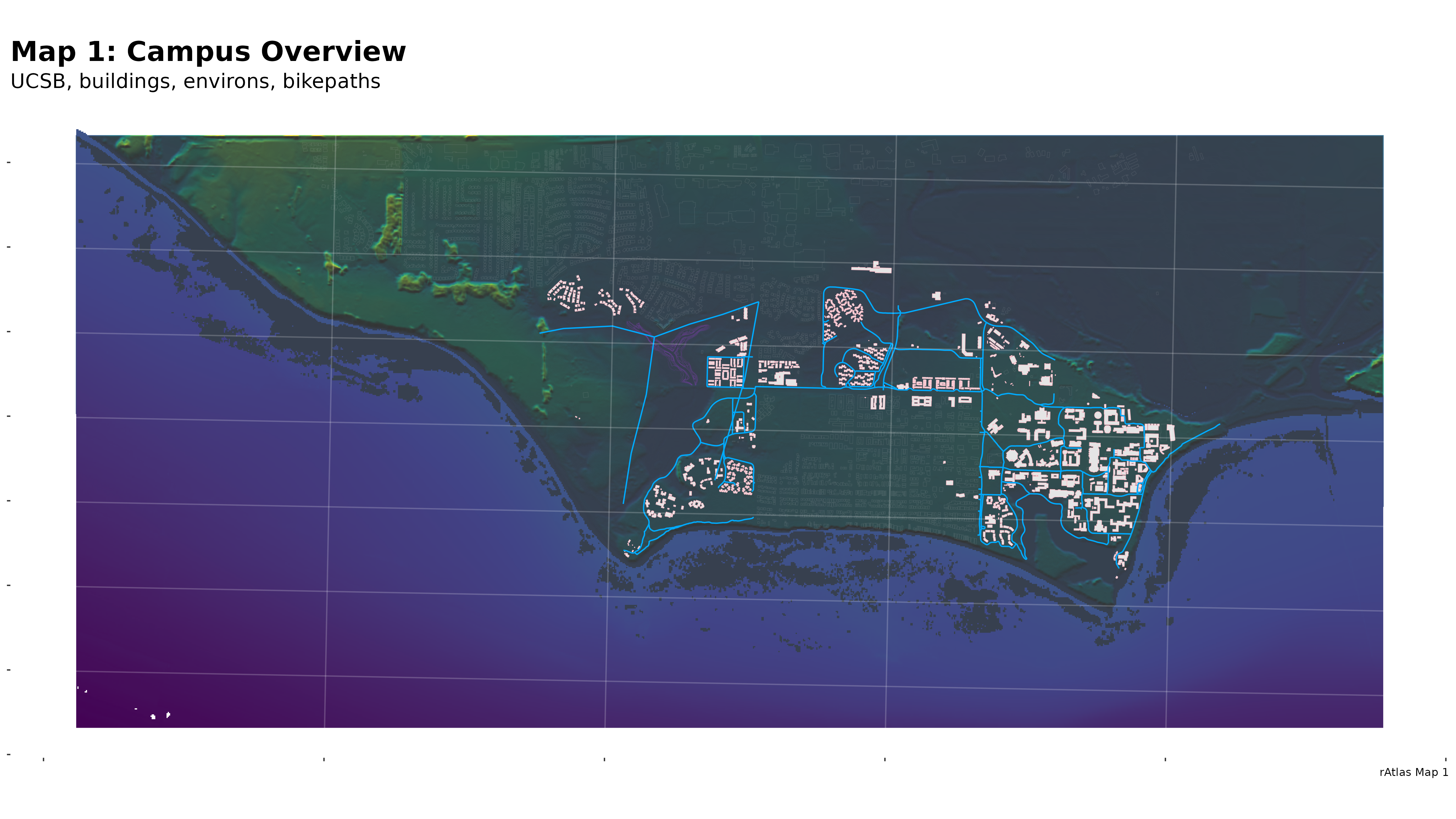
# map 1
# Wide overview of campus

library(tidyverse)
# library(raster)
library(terra)
library(sf)
library(scales)

# clean the environment and hidden objects
rm(list=ls())

gg_labelmaker <- function(plot_num){
  gg_title <- c("Map:", current_sheet, " ggplot:", plot_num)
  plot_text <- paste(gg_title, collapse=" " )
  print(plot_text)
  current_ggplot <<- plot_num
  return(plot_text)
}


# make our ggtitles automagically #######
# set map number
current_sheet <- 1
# set ggplot counter
current_ggplot <- 0

# every ggtitle() or labs() should be:
# ggtitle(gg_labelmaker(current_ggplot+1))
# end automagic ggtitle           #######


# we will use this to make the graticule and axes
my_theme <-   theme(axis.title.x=element_blank(), 
                    axis.title.y=element_blank(), 
                    axis.text.x=element_blank(), 
                    axis.text.y=element_blank(), 
                    legend.position="none", 
                    panel.ontop=TRUE,
                    panel.grid.major = element_line(color = "#FFFFFF33"),
                    panel.background = element_blank()) 




# add vector layers
buildings <- st_read("source_data/campus_buildings/Campus_Buildings.shp")
iv_buildings <- st_read("source_data/iv_buildings/iv_buildings/CA_Structures_ExportFeatures.shp")
# walkways <- ???
bikeways <- st_read("source_data/icm_bikes/bike_paths/bikelanescollapsedv8.shp")
habitat <- st_read("source_data/NCOS_Shorebird_Foraging_Habitat/NCOS_Shorebird_Foraging_Habitat.shp")
ncos_trails <- st_read("source_data/ncos_trails/ncos_multiuse_trails.geojson")


# basic terra plots
# $geometry does just the shape.
plot(buildings$geometry)
plot(iv_buildings$geometry)
plot(bikeways$geometry)
plot(habitat$geometry)
plot(ncos_trails$geometry)


# overlays as in episode 8

# #1 
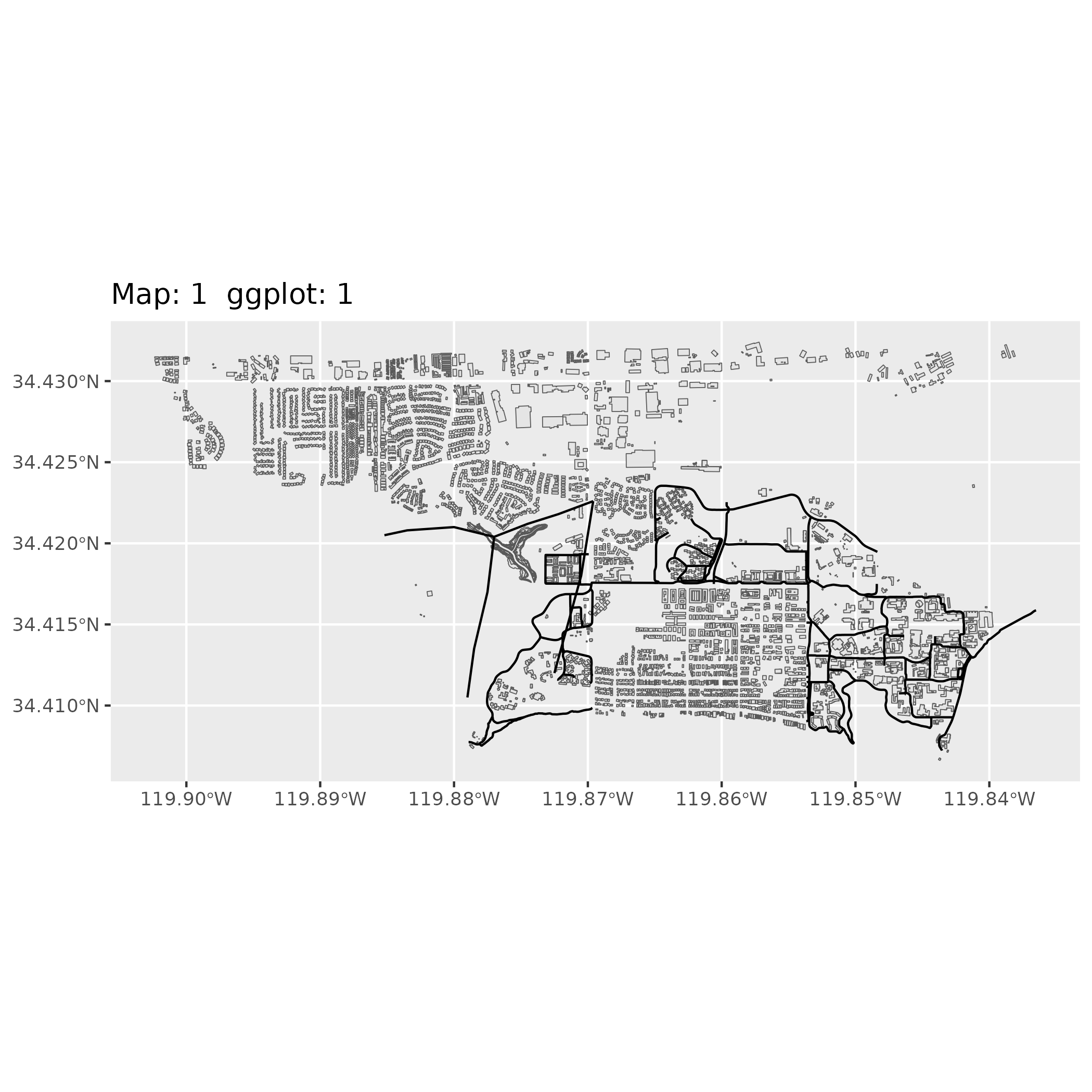
ggplot() +
  geom_sf(data=habitat) +
  geom_sf(data=buildings) +
  geom_sf(data=iv_buildings) +
  geom_sf(data=bikeways) +
  geom_sf(data=ncos_trails) +
  ggtitle(gg_labelmaker(current_ggplot+1)) +
  coord_sf()

ggsave("images/map1.1.png", plot=last_plot())

# don't forget you have a theme to use
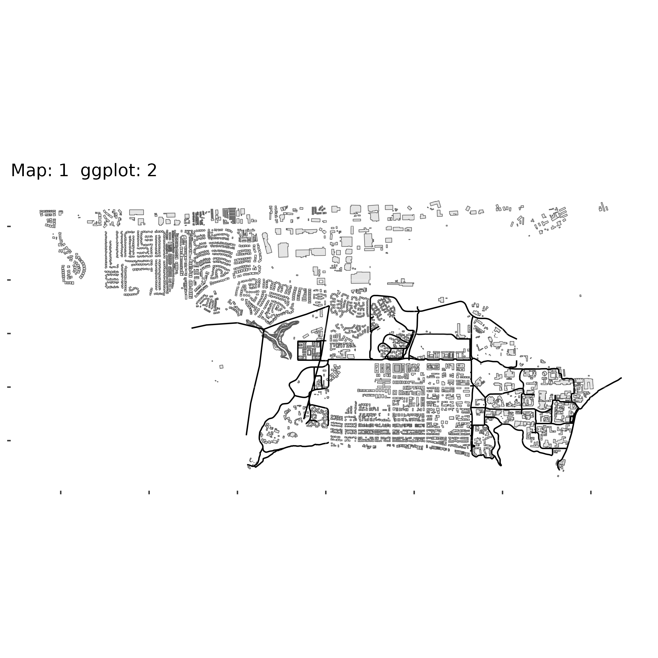
ggplot() +
  geom_sf(data=habitat) +
  geom_sf(data=buildings) +
  geom_sf(data=iv_buildings) +
  geom_sf(data=bikeways)  +
  geom_sf(data=ncos_trails) +
  my_theme +
  ggtitle(gg_labelmaker(current_ggplot+1)) +
  coord_sf()

ggsave("images/map1.2.png", plot=last_plot())



# which buildings are on top?
# the last ones added
# #2 
ggplot() +
  geom_sf(data=habitat, color="yellow") +
  geom_sf(data=iv_buildings, color="pink") +
  geom_sf(data=buildings) +
  geom_sf(data=bikeways, color="blue") +
  geom_sf(data=ncos_trails, color="blue") +
  my_theme +
  ggtitle(gg_labelmaker(current_ggplot+1)) +
  coord_sf()


# so visually let's put the non-campus gray
# buildings below our campus buildings

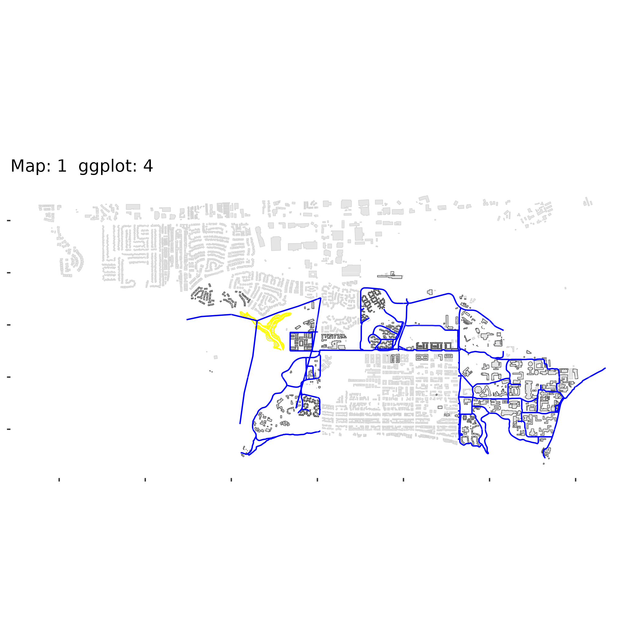
ggplot() +
  geom_sf(data=habitat, color="yellow") +
  geom_sf(data=iv_buildings, color="light gray") +
  geom_sf(data=buildings) +
  geom_sf(data=bikeways, color="blue") +
  geom_sf(data=ncos_trails, color="blue") +
  my_theme +
    ggtitle(gg_labelmaker(current_ggplot+1)) +
  coord_sf() 
  
ggsave("images/1.2.png", plot=last_plot())


# the background setup is bathymetry and topography
# mashed together

# We'll need some bins
# best coast line bins from ep 2
# from ep 2, these are best sea level bins:
custom_bins <- c(-3, 4.9, 5, 7.5, 10, 25, 40, 70, 100, 150, 200)



campus_DEM <- rast("source_data/campus_DEM.tif") 
crs(campus_DEM)

# does bathymetry still needs to be re-projected in order to overlay?
campus_bath <- rast("source_data/SB_bath.tif") 
crs(campus_bath)

# can't overlay them because they are different CRS's
# that's part of the narrative of the lesson.
plot(campus_DEM)
plot(campus_bath)


campus_projection <- crs(campus_DEM)

campus_bath <- project(campus_bath, campus_projection)
plot(campus_DEM)
plot(campus_bath)

crs(campus_DEM) == crs(campus_bath)

#################################
# Julien solved this in ep_4
# for these files, CRS, extent, and resolution all 
# need to be made to match:


# do they have the same projections?
crs(campus_DEM) == crs(campus_bath)

# do they have the same extents?
ext(campus_DEM) == ext(campus_bath)


campus_bath <- crop(x=campus_bath, y=campus_DEM)
plot(campus_bath)
crs(campus_bath)

# save campus bathymetry here
writeRaster(campus_bath, "output_data/campus_bath_epsg2874.tif", filetype="GTiff", overwrite=TRUE)

# make dataframes
campus_DEM_df <- as.data.frame(campus_DEM, xy=TRUE) %>%
  rename(elevation = greatercampusDEM_1_1) # rename to match code later
str(campus_DEM_df)

campus_bath_df <- as.data.frame(campus_bath, xy=TRUE) %>%
  rename(bathymetry = Bathymetry_2m_OffshoreCoalOilPoint)
str(campus_bath_df)

sea_level <- campus_DEM - 5

# Set values below or equal to 0 to NA
sea_level_0 <- app(sea_level, function(x) ifelse(x <=0, NA, x))

# Note: this remove some values in the marsh that are below 0
# we are going to want those back later 

# Make it a data frame and rebinned
sea_level_df <- as.data.frame(sea_level_0, xy=TRUE) %>% 
  rename(elevation = lyr.1) %>%
  mutate(binned = cut(elevation, breaks=custom_bins))

# to make our scale make sense, we can do 
# raster math 
# how would I do this with overlay?
ggplot() + 
  geom_raster(data = sea_level_df, aes(x=x, y=y, fill = binned)) + 
  my_theme +
    ggtitle(gg_labelmaker(current_ggplot+1)) +
  coord_sf()

summary(sea_level_df)
custom_sea_bins <- c(-8, -.1, .1, 3, 5, 7.5, 10, 25, 40, 70, 100, 150, 200)

sea_level_df <- sea_level_df %>% 
  mutate(binned = cut(elevation, breaks=custom_sea_bins))


length(custom_sea_bins)

# now sea level is zero.
ggplot() + 
  geom_raster(data = sea_level_df, aes(x=x, y=y, fill = binned)) +
  my_theme +
  ggtitle(gg_labelmaker(current_ggplot+1)) +
  coord_sf()

# if we overlay, we should get the same result as at the 
# end of (episode 1?).
ggplot() +
  geom_raster(data = campus_DEM_df, aes(x=x, y=y, fill = elevation)) +
  geom_raster(data = campus_bath_df, aes(x=x, y=y, fill = bathymetry)) +
  scale_fill_viridis_c(na.value="NA") +
  my_theme +
  ggtitle(gg_labelmaker(current_ggplot+1), subtitle = "Does the ovlerlay work?") +
  coord_sf()



# add custom bins to each.
# these were based on experimentation
custom_DEM_bins <- c(-3, -.01, .01, 2, 3, 4, 5, 10, 40, 200)
campus_DEM_df <- campus_DEM_df %>% 
  mutate(binned_DEM = cut(elevation, breaks = custom_DEM_bins))

str(campus_DEM_df)

custom_bath_bins <- c(1, -5, -15, -35, -45, -55, -60, -65, -75, -100, -125)
str(custom_bath_bins)

str(campus_bath_df)

campus_bath_df <- campus_bath_df %>% 
  mutate(binned_bath = cut(bathymetry, breaks =custom_bath_bins))

str(campus_bath_df)
str(campus_DEM_df)

# overlays works!!!!!
ggplot() + 
  geom_raster(data = campus_bath_df, aes(x=x, y=y, fill = binned_bath)) +
  scale_fill_manual(values = terrain.colors(10)) +
  geom_raster(data=campus_DEM_df, aes(x=x, y=y, fill = binned_DEM)) +
  scale_fill_manual(values = terrain.colors(19)) +
  my_theme +
  ggtitle(gg_labelmaker(current_ggplot+1), subtitle = "overlay works!") +
  coord_quickmap()

# switch the order
# Not sure how color scheme gets on both layers
ggplot() +
    geom_raster(data = campus_DEM_df, aes(x=x, y=y, fill = binned_DEM)) +
    geom_raster(data = campus_bath_df, aes(x=x, y=y, fill = binned_bath)) +
    scale_fill_manual(values = terrain.colors(19)) +
  my_theme +
  ggtitle(gg_labelmaker(current_ggplot+1)) +
  coord_quickmap()

ggplot() +
  geom_raster(data = campus_DEM_df, aes(x=x, y=y, fill = elevation)) +
  geom_raster(data = campus_bath_df, aes(x=x, y=y, fill = bathymetry)) +
        scale_fill_viridis_c(na.value="NA") +
  my_theme +
  ggtitle(gg_labelmaker(current_ggplot+1)) +
  coord_quickmap()
  
# create batho-topo
# while we are here, we should make 
# one DEM that is both bathymetry and elevation
# by combining campus_DEM and sea_level_0
# this is also in episode 9
# but ... does batho_topo plot the same?


plot(campus_bath)
plot(sea_level_0)

crs(campus_bath) == crs(sea_level_0)

# they have different resolutions
res(campus_bath)
res(sea_level_0)

campus_bath_20m <- resample(campus_bath, sea_level_0)

res(sea_level_0) 
res(campus_bath_20m)

campus_bathotopo <- merge(campus_bath_20m, sea_level_0)

plot(campus_bathotopo)
writeRaster(campus_bathotopo, "output_data/campus_bathotopo.tif", overwrite=TRUE)
# end batho-topo
# even though we don't do anything with it here in map 1
# ######

  
# overlay the vectors
# they won't overlay because
# you need to re-project the vectors
ggplot() +
  geom_raster(data = campus_DEM_df, aes(x=x, y=y, fill = elevation)) +
  geom_raster(data = campus_bath_df, aes(x=x, y=y, fill = bathymetry)) +
  scale_fill_viridis_c(na.value="NA") +
  geom_sf(data=habitat, color="yellow") +
  geom_sf(data=buildings) +
  geom_sf(data=bikeways, color="blue") +
  geom_sf(data=ncos_trails, color="blue") +
  my_theme +
  ggtitle(gg_labelmaker(current_ggplot+1)) +
    coord_sf()

# reproject the vectors
buildings <- st_transform(buildings, crs(campus_DEM))
iv_buildings <- st_transform(iv_buildings, crs(campus_DEM))
bikeways <- st_transform(bikeways, crs(campus_DEM))
habitat <- st_transform(habitat, crs(campus_DEM))
ncos_trails <- st_transform(ncos_trails, crs(campus_DEM))

# now the overlays work
ggplot() +
  geom_raster(data = campus_DEM_df, aes(x=x, y=y, fill = elevation)) +
  geom_raster(data = campus_bath_df, aes(x=x, y=y, fill = bathymetry)) +
  scale_fill_viridis_c(na.value="NA") +
  geom_sf(data=habitat, color="yellow") +
  geom_sf(data=buildings) +
  geom_sf(data=bikeways, color="blue") +
  geom_sf(data=ncos_trails, color="blue") +
  my_theme +
  ggtitle(gg_labelmaker(current_ggplot+1)) +
  coord_sf()


# bring back the hillshade
# open file from ep1-2
# and maybe put it on top of batho_topo since you never use that one?

campus_hillshade_df <- 
  rast("source_data/campus_hillshade.tif") %>% 
  as.data.frame(xy = TRUE) %>% 
  rename(campus_hillshade = hillshade) # rename to match code later

str(campus_hillshade_df)


#update color scheme for contrast 
# +hillshade
# trying with the scales library to shorten the x, y to 2 decimals
ggplot() +
  geom_raster(data = campus_DEM_df, aes(x=x, y=y, fill = elevation)) +
  geom_raster(data = campus_hillshade_df, aes(x=x, y=y, alpha = campus_hillshade), show.legend = FALSE) +
  geom_raster(data = campus_bath_df, aes(x=x, y=y, fill = bathymetry)) +
  scale_fill_viridis_c(na.value="NA")+ 
  scale_y_continuous(labels = number_format(accuracy = 0.01)) +
  geom_sf(data=iv_buildings, color=alpha("light gray", .1), fill=NA) +
  geom_sf(data=buildings, color ="hotpink") +
  geom_sf(data=habitat, color="darkorchid1") +
  geom_sf(data=bikeways, color="#00abff") +
  geom_sf(data=ncos_trails, color="#00abff") +
  my_theme +
  ggtitle(gg_labelmaker(current_ggplot+1)) +
  coord_sf()


# next we need to refine the plot and labels
# Not a publication ready graphic (yet) ~episode 13
# customize the x and y graticule to be xx.xx and smaller -> number_format()
# remove the x and y axis labels -> axis.title.x/y = element_blank()
# customize the legend title to include units of elevation -> guide_legend()
gg_title_string <- gg_labelmaker(current_ggplot)
gg_title_string
# #  
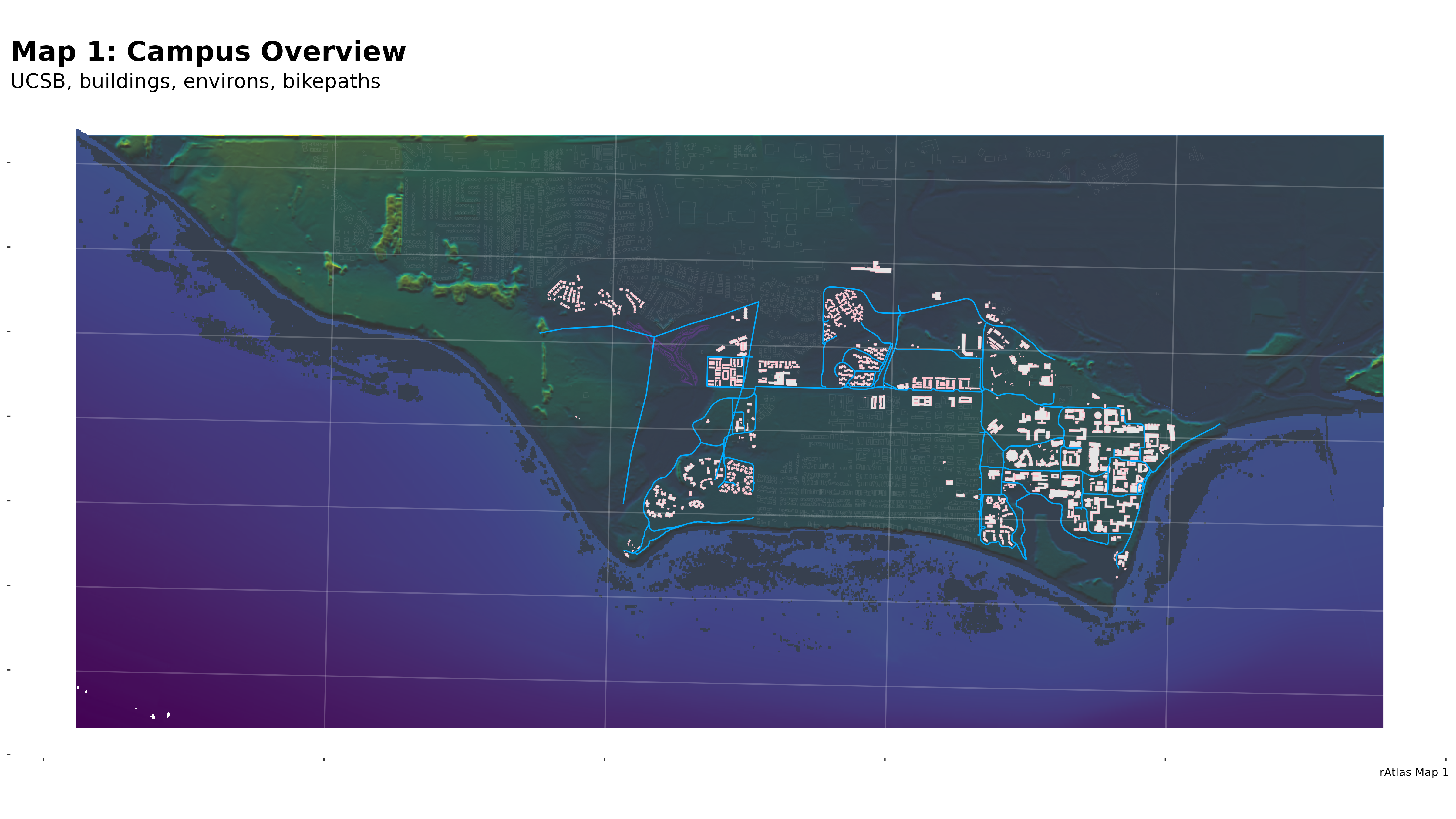
final_ggplot <- ggplot() +
  geom_raster(data = campus_DEM_df, aes(x=x, y=y, fill = elevation)) +
  geom_raster(data = campus_hillshade_df, aes(x=x, y=y, alpha = campus_hillshade)) +
  geom_raster(data = campus_bath_df, aes(x=x, y=y, fill = bathymetry)) +
  scale_y_continuous(labels = number_format(accuracy = 0.01)) +
  scale_fill_viridis_c(na.value="NA", guide = guide_legend("bathymetry / elevation (US ft)"))+
  geom_sf(data=iv_buildings, color=alpha("light gray", .1), fill=NA) +
  geom_sf(data=buildings, color ="pink") +
  geom_sf(data=habitat, color=alpha("darkorchid1", .1), fill=NA) +
  geom_sf(data=bikeways, color="#00abff") +
  geom_sf(data=ncos_trails, color="#00abff") +
  labs(title=gg_title_string, 
       subtitle="UCSB, buildings, environs, bikepaths",
       caption = "rAtlas Map 1") + 
  my_theme +
  coord_sf()


# Modern NCOS multi-use trails added to bridge the network across NCOS

final_ggplot
ggsave("images/map1.11.png", width = 16, height = 9, plot=final_ggplot)
ggsave("final_output/map_01.png", width = 16, height = 9, plot=final_ggplot)