# map 4
# clean the environment and hidden objects

rm(list = ls())

library(sf)
library(terra)
library(tidyterra)
library(geojsonsf)
library(ggplot2)
library(dplyr)

# set map number
current_sheet <- 4
# set ggplot counter
current_ggplot <- 0

# our auto ggtitle maker
gg_labelmaker <- function(plot_num) {
  gg_title <- c("Map:", current_sheet, " ggplot:", plot_num)
  plot_text <- paste(gg_title, collapse = " ")
  print(plot_text)
  current_ggplot <<- plot_num
  return(plot_text)
}
# every ggtitle should be:
# ggtitle(gg_labelmaker(current_ggplot+1))
# end automagic ggtitle


# ############################
# Map 4
# Zoom 2: Bite of California

# use campus CRS as standard
campus_DEM <- rast("source_data/campus_DEM.tif")
crs(campus_DEM)
campus_crs <- crs(campus_DEM)

# the extent of the campus_DEM
# is the zoom 3 indicator,
zoom_3_extent <- ext(campus_DEM) %>% vect()
crs(zoom_3_extent) <- campus_crs


# Get the west coast DEM and
# Crop it to zoom 2 AOI
# socal_aoi.geojson
zoom_2 <- rast("source_data/dem90_hf/dem90_hf.tif")
plot(zoom_2)

# AOI came from a Planet harvest that we did
zoom_2_crop_extent <- geojson_sf("source_data/socal_aoi.geojson")
zoom_2_crop_extent <- vect(zoom_2_crop_extent)

crs(zoom_2_crop_extent) == crs(zoom_2)

# project it to match west_us
# this will also 'rotate' southern california
# when we crop it, making it visually more readable
zoom_2_crop_extent <- project(zoom_2_crop_extent, crs(zoom_2))
crs(zoom_2_crop_extent) == crs(zoom_2)

# plot them together
# to confirm that's the correct extent
# that you want to crop to
plot(zoom_2)
polys(zoom_2_crop_extent)

# now crop to that extent
zoom_2_cropped <- crop(x = zoom_2, y = zoom_2_crop_extent)
plot(zoom_2_cropped)
# we need water! #####################

# batho-topo / SB_bath won't be big enough
bath <- rast("source_data/SB_bath.tif")
plot(bath)


# let's try the global hillshade?
# is it a hillshade? it looks like it.
zoom_2_water <- rast("source_data/global_raster/GRAY_HR_SR_OB.tif")
plot(zoom_2_water)

zoom_2_crop_extent <- project(zoom_2_crop_extent, crs(zoom_2_water))
zoom_2_water <- crop(x = zoom_2_water, y = (zoom_2_crop_extent))
plot(zoom_2_water)

crs(zoom_2_water) == crs(zoom_2_cropped)
zoom_2_water <- project(zoom_2_water, crs(zoom_2_cropped))
crs(zoom_2_water) == crs(zoom_2_cropped)


# make dataframes for ggplotting
zoom_2_DEM_df <- as.data.frame(zoom_2_cropped, xy = TRUE)
zoom_2_hillshade_df <- as.data.frame(zoom_2_water, xy = TRUE)
str(zoom_2_hillshade_df)
str(zoom_2_DEM_df)


# let's START
# with the graticule that we ended map 3 with:

ggplot() +
  geom_raster(
    data = zoom_2_hillshade_df,
    aes(x = x, y = y, alpha = GRAY_HR_SR_OB)
  ) +
  scale_alpha(range = c(0.05, 0.55), guide = "none") +
  coord_sf() +
  theme(
    axis.title.x = element_blank(),
    axis.title.y = element_blank(),
    legend.position = "none",
    panel.ontop = TRUE,
    panel.grid.major = element_line(color = "#FFFFFF33"),
    panel.background = element_blank()
  ) +
  ggtitle("Map 4: zm 2: hillshade", subtitle = gg_labelmaker(current_ggplot + 1))

ggplot() +
  geom_raster(
    data = zoom_2_DEM_df,
    aes(x = x, y = y, fill = dem90_hf)
  ) +
  scale_fill_viridis_c() +
  coord_sf() +
  theme(
    axis.title.x = element_blank(),
    axis.title.y = element_blank(),
    legend.position = "none",
    panel.ontop = TRUE,
    panel.grid.major = element_line(color = "#FFFFFF33"),
    panel.background = element_blank()
  ) +
  ggtitle("Map 4: zm 2: dem", subtitle = gg_labelmaker(current_ggplot + 1))

# try to overlay
ggplot() +
  geom_raster(
    data = zoom_2_DEM_df,
    aes(x = x, y = y, fill = dem90_hf)
  ) +
  scale_fill_viridis_c() +
  geom_raster(
    data = zoom_2_hillshade_df,
    aes(x = x, y = y, alpha = GRAY_HR_SR_OB)
  ) +
  scale_alpha(range = c(0.05, 0.55), guide = "none") +
  coord_sf() +
  theme(
    axis.title.x = element_blank(),
    axis.title.y = element_blank(),
    legend.position = "none",
    panel.ontop = TRUE,
    panel.grid.major = element_line(color = "#FFFFFF33"),
    panel.background = element_blank()
  ) +
  ggtitle("Map 4: zm 2: Overlay test", subtitle = gg_labelmaker(current_ggplot + 1))

# so close!!!!!!


# now I need the next zoom indicator
# I need to project that too.
crs(zoom_3_extent) == crs(zoom_2_cropped)
zoom_3_extent <- project(zoom_3_extent, zoom_2_cropped)
plot(zoom_3_extent)

ggplot() +
  geom_raster(
    data = zoom_2_DEM_df,
    aes(x = x, y = y, fill = dem90_hf)
  ) +
  scale_fill_viridis_c() +
  geom_raster(
    data = zoom_2_hillshade_df,
    aes(x = x, y = y, alpha = GRAY_HR_SR_OB)
  ) +
  scale_alpha(range = c(0.05, 0.55), guide = "none") +
  coord_sf() +
  theme(
    axis.title.x = element_blank(),
    axis.title.y = element_blank(),
    legend.position = "none",
    panel.ontop = TRUE,
    panel.grid.major = element_line(color = "#FFFFFF33"),
    panel.background = element_blank()
  ) +
  ggtitle("Map 4: zm 2: Overlay test", subtitle = gg_labelmaker(current_ggplot + 1))


# add the zoom indicator to the ggplot
ggplot() +
  geom_spatvector(data = zoom_3_extent, color = "red", fill = NA, lwd = 1) +
  theme(
    panel.grid.major = element_line(color = "#FFFFFF33"),
    panel.background = element_blank()
  ) +
  coord_sf()

# now that I've added tidyterra, both the above geom_spatvecor
# and the below geom_sf work

ggplot() +
  geom_raster(
    data = zoom_2_DEM_df,
    aes(x = x, y = y, fill = dem90_hf)
  ) +
  scale_fill_viridis_c() +
  geom_raster(
    data = zoom_2_hillshade_df,
    aes(x = x, y = y, alpha = GRAY_HR_SR_OB)
  ) +
  scale_alpha(range = c(0.05, 0.55), guide = "none") +
  #  geom_spatvector(data=zoom_3_extent, color="red", fill=NA, lwd=1)+
  geom_sf(data = zoom_3_extent, color = "red", fill = NA, lwd = 1) +
  coord_sf() +
  theme(
    axis.title.x = element_blank(),
    axis.title.y = element_blank(),
    legend.position = "none",
    panel.ontop = TRUE,
    panel.grid.major = element_line(color = "#FFFFFF33"),
    panel.background = element_blank()
  ) +
  ggtitle("Map 4: zm 2: Overlay with Indicator", subtitle = gg_labelmaker(current_ggplot + 1))


ggplot() +
  geom_raster(
    data = zoom_2_DEM_df,
    aes(x = x, y = y, fill = dem90_hf)
  ) +
  scale_fill_viridis_c() +
  geom_raster(
    data = zoom_2_hillshade_df,
    aes(x = x, y = y, alpha = GRAY_HR_SR_OB)
  ) +
  scale_alpha(range = c(0.05, 0.55), guide = "none") +
  geom_sf(data = zoom_3_extent, color = "red", fill = NA, lwd = 1) +
  theme(
    axis.title.x = element_blank(),
    axis.title.y = element_blank(),
    legend.position = "none",
    panel.ontop = TRUE,
    panel.grid.major = element_line(color = "#FFFFFF33"),
    panel.background = element_blank()
  ) +
  coord_sf() +
  ggtitle("Map 4: zm 2: Different hillshade", subtitle = gg_labelmaker(current_ggplot + 1))


# 'california populated places'
# which is census data
# for the sake of a nice vizualization
places <- vect("source_data/tl_2023_06_place/tl_2023_06_place.shp")
plot(places)
crs(places) == campus_crs
places <- project(places, campus_crs)

# places still not showing up
#---------------------------------------

str(zoom_2_hillshade_df)
# For zoom 2, places does not overlay nicely.
# this is another CRS error
ggplot() +
  geom_raster(
    data = zoom_2_DEM_df,
    aes(x = x, y = y, fill = dem90_hf)
  ) +
  scale_fill_viridis_c() +
  geom_raster(
    data = zoom_2_hillshade_df,
    aes(x = x, y = y, alpha = GRAY_HR_SR_OB)
  ) +
  scale_alpha(range = c(0.05, 0.5), guide = "none") +
  geom_spatvector(data = places, fill = "gray") +
  geom_spatvector(data = zoom_3_extent, color = "red", fill = NA) +
  theme(
    axis.title.x = element_blank(),
    axis.title.y = element_blank(),
    legend.position = "none",
    panel.ontop = TRUE,
    panel.grid.major = element_line(color = "#FFFFFF33"),
    panel.background = element_blank()
  ) +
  coord_sf() +
  ggtitle("Map 4: zm 2: Zoom test 2", subtitle = gg_labelmaker(current_ggplot + 1))

crs(zoom_2_cropped) == campus_crs
crs(zoom_2_water) == campus_crs
crs(zoom_2_cropped) == crs(zoom_2_water)
crs(places) == campus_crs
# places is the one to reproject right now.

places <- project(places, crs(zoom_2_cropped))

ggplot() +
  geom_raster(
    data = zoom_2_DEM_df,
    aes(x = x, y = y, fill = dem90_hf)
  ) +
  scale_fill_viridis_c() +
  geom_raster(
    data = zoom_2_hillshade_df,
    aes(x = x, y = y, alpha = GRAY_HR_SR_OB)
  ) +
  scale_alpha(range = c(0.05, 0.5), guide = "none") +
  geom_spatvector(data = places, fill = "gray") +
  geom_spatvector(data = zoom_3_extent, color = "red", fill = NA) +
  theme(
    axis.title.x = element_blank(),
    axis.title.y = element_blank(),
    legend.position = "none",
    panel.ontop = TRUE,
    panel.grid.major = element_line(color = "#FFFFFF33"),
    panel.background = element_blank()
  ) +
  coord_sf() +
  ggtitle("Map 4: zm 2: re-projected places", subtitle = gg_labelmaker(current_ggplot + 1))

# this plots, but to the full extent of california.
# we are gonna need to crop places

# this also plots, but at the full extent of california.

zoom_2_places <- crop(places, zoom_2_cropped)

ggplot() +
  geom_raster(
    data = zoom_2_DEM_df,
    aes(x = x, y = y, fill = dem90_hf)
  ) +
  scale_fill_viridis_c() +
  geom_raster(
    data = zoom_2_hillshade_df,
    aes(x = x, y = y, alpha = GRAY_HR_SR_OB)
  ) +
  scale_alpha(range = c(0.05, 0.5), guide = "none") +
  geom_spatvector(data = zoom_2_places, fill = "gray") +
  geom_spatvector(data = zoom_3_extent, color = "red", fill = NA) +
  theme(
    axis.title.x = element_blank(),
    axis.title.y = element_blank(),
    legend.position = "none",
    panel.ontop = TRUE,
    panel.grid.major = element_line(color = "#FFFFFF33"),
    panel.background = element_blank()
  ) +
  coord_sf() +
  ggtitle("Map 4: zm 2: re-projected places", subtitle = gg_labelmaker(current_ggplot + 1))

# it plots!!!!! but ugly.
ggsave("images/map4.png", width = 3, height = 4, plot = last_plot(), bg = "white")

# how can I make the fill transparent?

ggplot() +
  geom_spatvector(data = zoom_2_places, color = "#D3D3D380", fill = "#D4D4D450") +
  coord_sf() +
  ggtitle("Map 4: zm 2: re-projected places", subtitle = gg_labelmaker(current_ggplot + 1))


# better
# and add places viz from map 3
ggplot() +
  geom_raster(
    data = zoom_2_DEM_df,
    aes(x = x, y = y, fill = dem90_hf)
  ) +
  scale_fill_viridis_c() +
  geom_raster(
    data = zoom_2_hillshade_df,
    aes(x = x, y = y, alpha = GRAY_HR_SR_OB)
  ) +
  scale_alpha(range = c(0.05, 0.5), guide = "none") +
  geom_spatvector(data = zoom_2_places, fill = "NA", color = "#EEEEEE33") +
  geom_spatvector(data = zoom_3_extent, color = "red", fill = NA) +
  theme_minimal() +
  theme(
    axis.title.x = element_blank(),
    axis.title.y = element_blank(),
    legend.position = "none",
    panel.ontop = TRUE,
    panel.grid.major = element_line(color = "#FFFFFF33"),
    panel.background = element_blank()
  ) +
  coord_sf() +
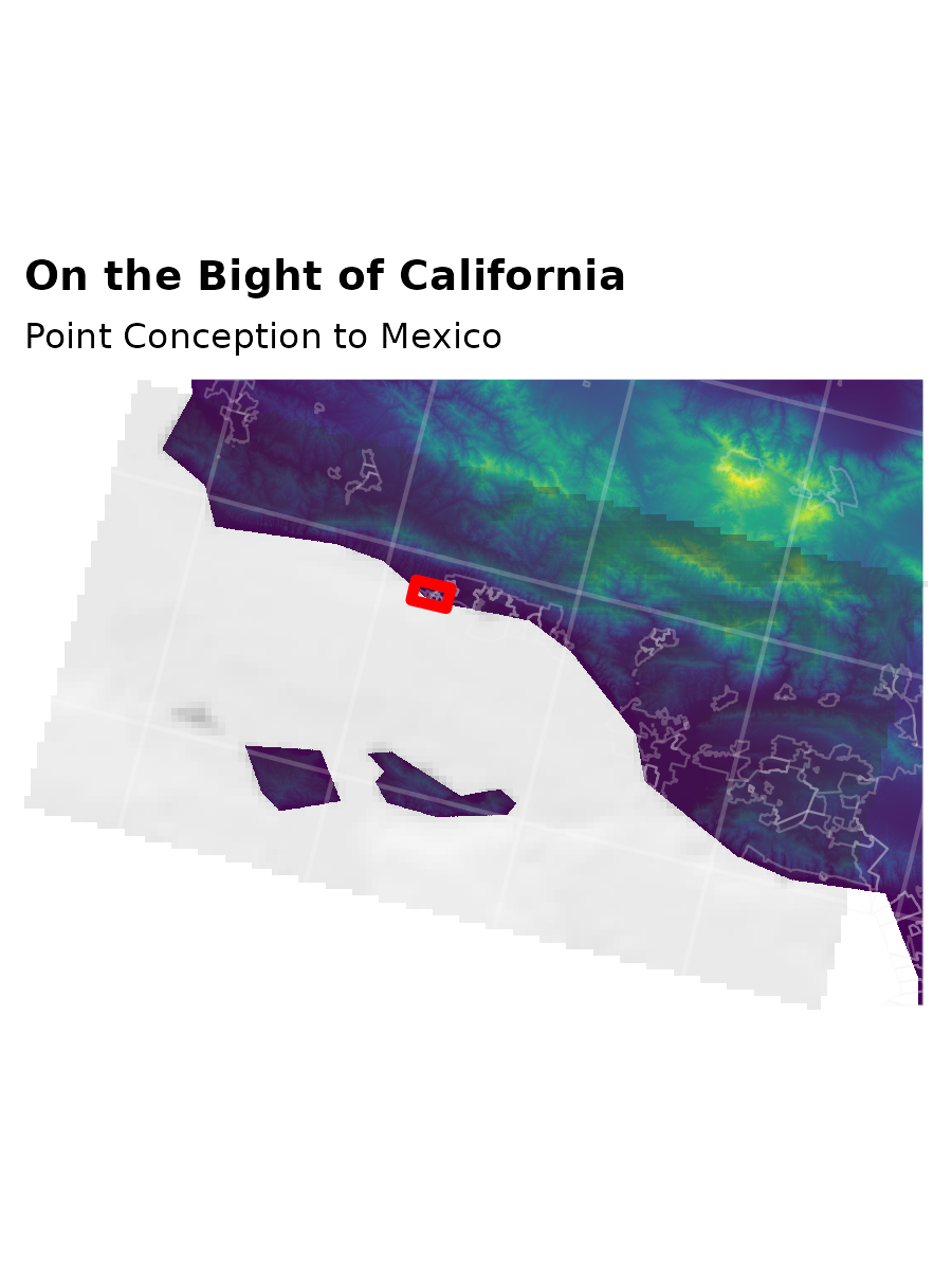
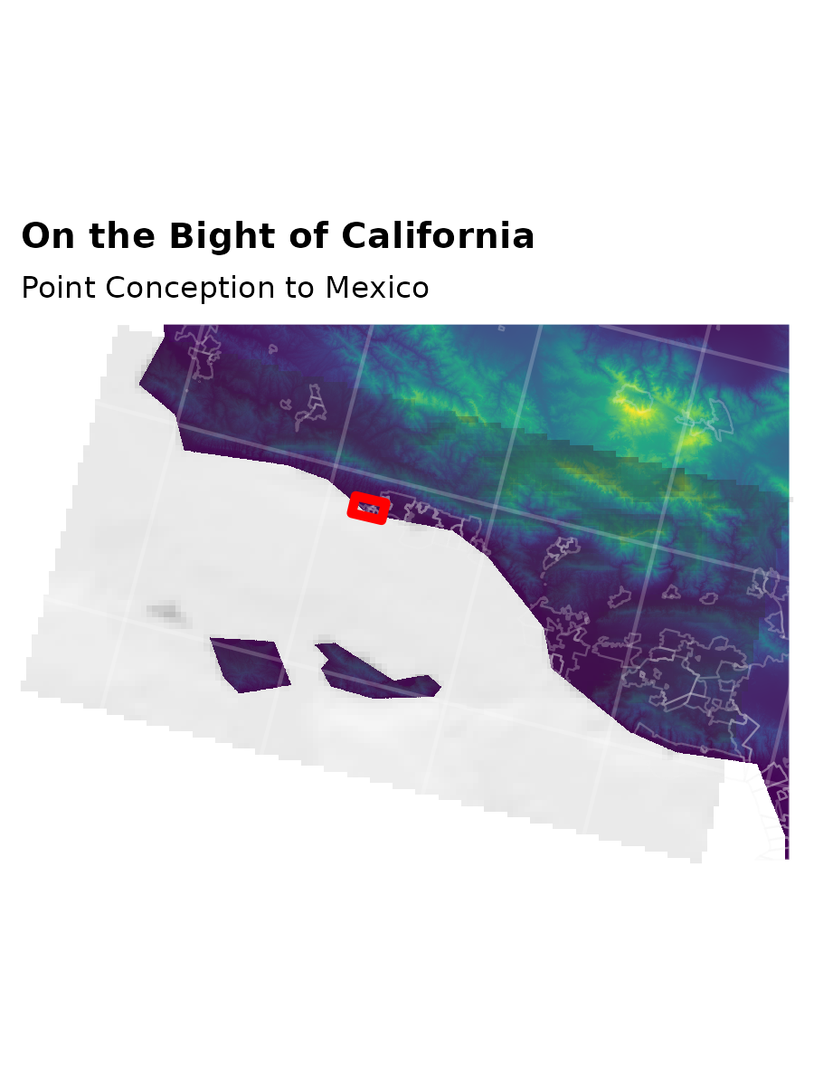
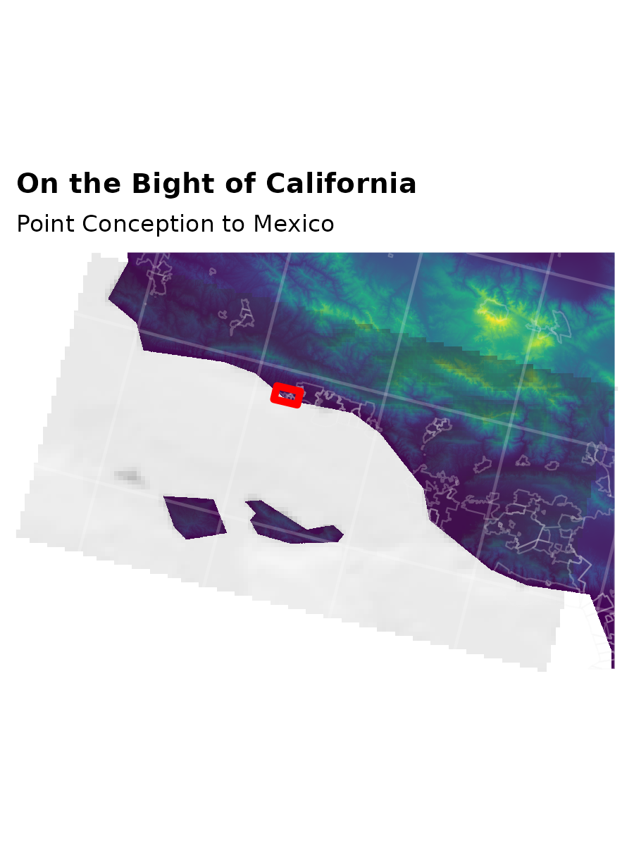
  ggtitle("Map 4: zm 2: The Bight of California", subtitle = gg_labelmaker(current_ggplot + 1))

# and a final one for saving
zoom_3_extent_proj <- project(zoom_3_extent, crs(zoom_2_cropped))

zoom_2_final_plot <- ggplot() +
  geom_raster(
    data = zoom_2_DEM_df,
    aes(x = x, y = y, fill = dem90_hf)
  ) +
  scale_fill_viridis_c(guide = "none") +
  geom_raster(
    data = zoom_2_hillshade_df,
    aes(x = x, y = y, alpha = GRAY_HR_SR_OB)
  ) +
  scale_alpha(range = c(0.05, 0.5), guide = "none") +
  geom_spatvector(data = zoom_2_places, fill = "NA", color = "#EEEEEE40", linewidth = 0.25) +
  geom_spatvector(data = zoom_3_extent_proj, color = "red", fill = NA, linewidth = 1.2) +
  theme_minimal() +
  theme(
    axis.title = element_blank(),
    axis.text = element_blank(),
    axis.ticks = element_blank(),
    legend.position = "none",
    panel.ontop = TRUE,
    panel.grid.major = element_line(color = "#FFFFFF33"),
    panel.background = element_blank()
  ) +
  coord_sf(expand = FALSE) +
  ggtitle("On the Bight of California",
    subtitle = "Point Conception to Mexico"
  )

zoom_2_final_plot

ggsave("images/map4.png", width = 3, height = 4, plot = zoom_2_final_plot, bg = "white")
ggsave("images/map_04.png", width = 3, height = 4, plot = zoom_2_final_plot, bg = "white")
ggsave("final_output/map_04.png", width = 3, height = 4, plot = zoom_2_final_plot, bg = "white")