# map 3-4-5 is a tryptic,
# that runs horizontally on top of map 7
# zooming in to campus
# ie: the zoom to Cali locator sheet

# each of the 3 maps is a grayscale alpha hillshade
# over (some color-scheme) DEMs,
# -- just as in the overlay episode --
#  -- which overlay episode Jonnie?     --


# clean the environment and hidden objects
rm(list = ls())

library(terra)
library(geojsonsf)
# library(sf)
library(ggplot2)
library(tidyterra)
library(dplyr)
# library(ggpubr)
# library(raster)

# make sure output window is 1x1
# because you muck with it a lot
par(mfrow = c(1, 1))

# We'll need a grayscale palette later
grays <- colorRampPalette(c("black", "white"))(255)

# set map number
current_sheet <- 3
# set ggplot counter
current_ggplot <- 0

# our auto ggtitle maker
gg_labelmaker <- function(plot_num) {
  gg_title <- c("Map:", current_sheet, " ggplot:", plot_num)
  plot_text <- paste(gg_title, collapse = " ")
  print(plot_text)
  current_ggplot <<- plot_num
  return(plot_text)
}
# every ggtitle should be:
# ggtitle(gg_labelmaker(current_ggplot+1))
# end automagic ggtitle           #######

# we will use this to make the graticule and axes
my_theme <- theme(
  axis.title.x = element_blank(),
  axis.title.y = element_blank(),
  axis.text.x = element_blank(),
  axis.text.y = element_blank(),
  legend.position = "none",
  panel.ontop = TRUE,
  panel.grid.major = element_line(color = "#FFFFFF33"),
  panel.background = element_blank()
)

# set up a local CRS to use throughout
campus_DEM <- rast("source_data/campus_DEM.tif")
campus_crs <- crs(campus_DEM)
str(campus_crs)


# #####################
# Map 3
# Zoom 1: west US overview

# hillshade:
world <- rast("source_data/global_raster/GRAY_HR_SR_OB.tif")
plot(world)

# dem:
zoom_1_dem <- rast("source_data/dem90_hf/dem90_hf.tif")
plot(zoom_1_dem)
# this is a bit too big later on. let's downsample it:
zoom_1_dem <- aggregate(zoom_1_dem, fact = 5)
plot(zoom_1_dem)

# and get our clipping extent
zoom_1_extent <- geojson_sf("source_data/cali_overview.geojson")
zoom_1_extent_vect <- vect(zoom_1_extent)
zoom_1_extent_vect
zoom_1_extent


# clip the world hillshade to zoom_1
zoom_1_hillshade <- crop(x = world, y = zoom_1_extent)
plot(zoom_1_hillshade)

crs(zoom_1_hillshade)
zoom_1_extent_vect <- project(x = zoom_1_extent_vect, y = zoom_1_hillshade)

# clip the dem
crs(zoom_1_dem) == crs(zoom_1_hillshade)
zoom_1_dem <- project(zoom_1_dem, crs(zoom_1_hillshade))
crs(zoom_1_dem) == crs(zoom_1_hillshade)

zoom_1_dem <- crop(x = zoom_1_dem, y = zoom_1_hillshade)

plot(zoom_1_dem)
plot(zoom_1_hillshade)


# we'll need this locator box socal_aoi.geojson
# is the next crop extent.
# it came from a Planet harvest that we did
zoom_2_crop_extent <- geojson_sf("source_data/socal_aoi.geojson")
zoom_2_crop_extent <- vect(zoom_2_crop_extent)


# now let's set up for ggplot
# and alphas
#################################################

# first check that projections match
crs(zoom_1_hillshade) == crs(zoom_1_dem)
crs(zoom_1_dem) == crs(zoom_2_crop_extent)
crs(zoom_1_hillshade) == crs(zoom_2_crop_extent)
# the rasters don't match the vector.
# but we still seem to be able to overlay.


# hillshade as ggplot
str(zoom_1_hillshade)
zoom_1_hillshade_df <- as.data.frame(zoom_1_hillshade, xy = TRUE)
colnames(zoom_1_hillshade_df)

zoom_1_hillshade_plot <- ggplot() +
  geom_raster(
    data = zoom_1_hillshade_df,
    aes(x = x, y = y, fill = GRAY_HR_SR_OB)
  ) +
  scale_fill_continuous() +
  coord_sf() +
  ggtitle("Zoom 1 Hillshade", subtitle = gg_labelmaker(current_ggplot + 1))

# zoom_1_hillshade_plot

# zoom 1 DEM as ggplot
str(zoom_1_dem)
zoom_1_dem_df <- as.data.frame(zoom_1_dem, xy = TRUE)
colnames(zoom_1_dem_df)

zoom_1_dem_plot <- ggplot() +
  geom_raster(
    data = zoom_1_dem_df,
    aes(x = x, y = y, fill = dem90_hf)
  ) +
  scale_fill_viridis_c() +
  coord_sf() +
  ggtitle("Zoom1 DEM", subtitle = gg_labelmaker(current_ggplot + 1))

# zoom_1_dem_plot


# hillshade as alpha
zoom_1_hillshade_plot <- ggplot() +
  geom_raster(
    data = zoom_1_hillshade_df,
    aes(x = x, y = y, alpha = GRAY_HR_SR_OB)
  ) +
  scale_alpha(range = c(0.3, 0.6), guide = "none") +
  coord_sf() +
  ggtitle("Zoom 1 Hillshade Alpha", subtitle = gg_labelmaker(current_ggplot + 1))

# zoom_1_hillshade_plot


# now overlay them
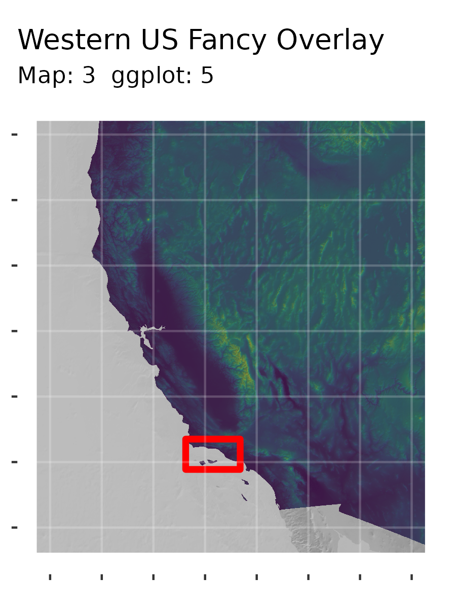
zoom_1_overlay_plot <- ggplot() +
  geom_raster(
    data = zoom_1_dem_df,
    aes(x = x, y = y, fill = dem90_hf)
  ) +
  scale_fill_viridis_c() +
  geom_raster(
    data = zoom_1_hillshade_df,
    aes(x = x, y = y, alpha = GRAY_HR_SR_OB)
  ) +
  scale_alpha(range = c(0.3, 0.6), guide = "none") +
  geom_spatvector(data = zoom_2_crop_extent, color = "red", lwd = 1.5, fill = NA) +
  coord_sf() +
  my_theme +
  ggtitle("Western US Fancy Overlay", subtitle = gg_labelmaker(current_ggplot + 1))
# zoom_1_overlay_plot


# the hillshade for the water is very subtle.
# zoom_1_overlay_plot

# add the graticule
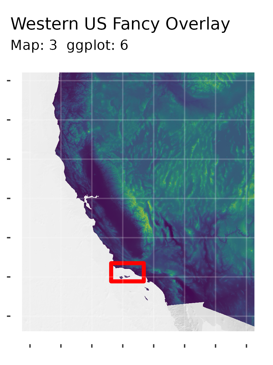
zoom_1_overlay_plot <- ggplot() +
  geom_raster(
    data = zoom_1_dem_df,
    aes(x = x, y = y, fill = dem90_hf)
  ) +
  scale_fill_viridis_c() +
  geom_raster(
    data = zoom_1_hillshade_df,
    aes(x = x, y = y, alpha = GRAY_HR_SR_OB)
  ) +
  scale_alpha(range = c(0.3, 0.6), guide = "none") +
  geom_spatvector(data = zoom_2_crop_extent, color = "red", lwd = 1.5, fill = NA) +
  my_theme +
  coord_sf() +
  ggtitle("Western US Fancy Overlay", subtitle = gg_labelmaker(current_ggplot + 1))

# zoom_1_overlay_plot
# ggsave("images/map3.1.png", width = 3, height = 4, plot = last_plot(), bg = "white")

# now seize control of labels
# zoom_1_overlay_plot
# ggsave("images/map3.2.png", width = 3, height = 4, plot = last_plot(), bg = "white")


# now let's add
# 'california populated places'
# which is census data
# for the sake of a nice vizualization
places <- vect("source_data/tl_2023_06_place/tl_2023_06_place.shp")
places <- project(places, crs(zoom_1_dem))
places <- crop(places, zoom_1_hillshade)
places_simple <- simplifyGeom(places, tolerance = 0.005)

# California state boundary polygon
cal_poly <- vect("source_data/california_boundary.geojson")
cal_poly <- project(cal_poly, crs(zoom_1_dem))

# now one to save
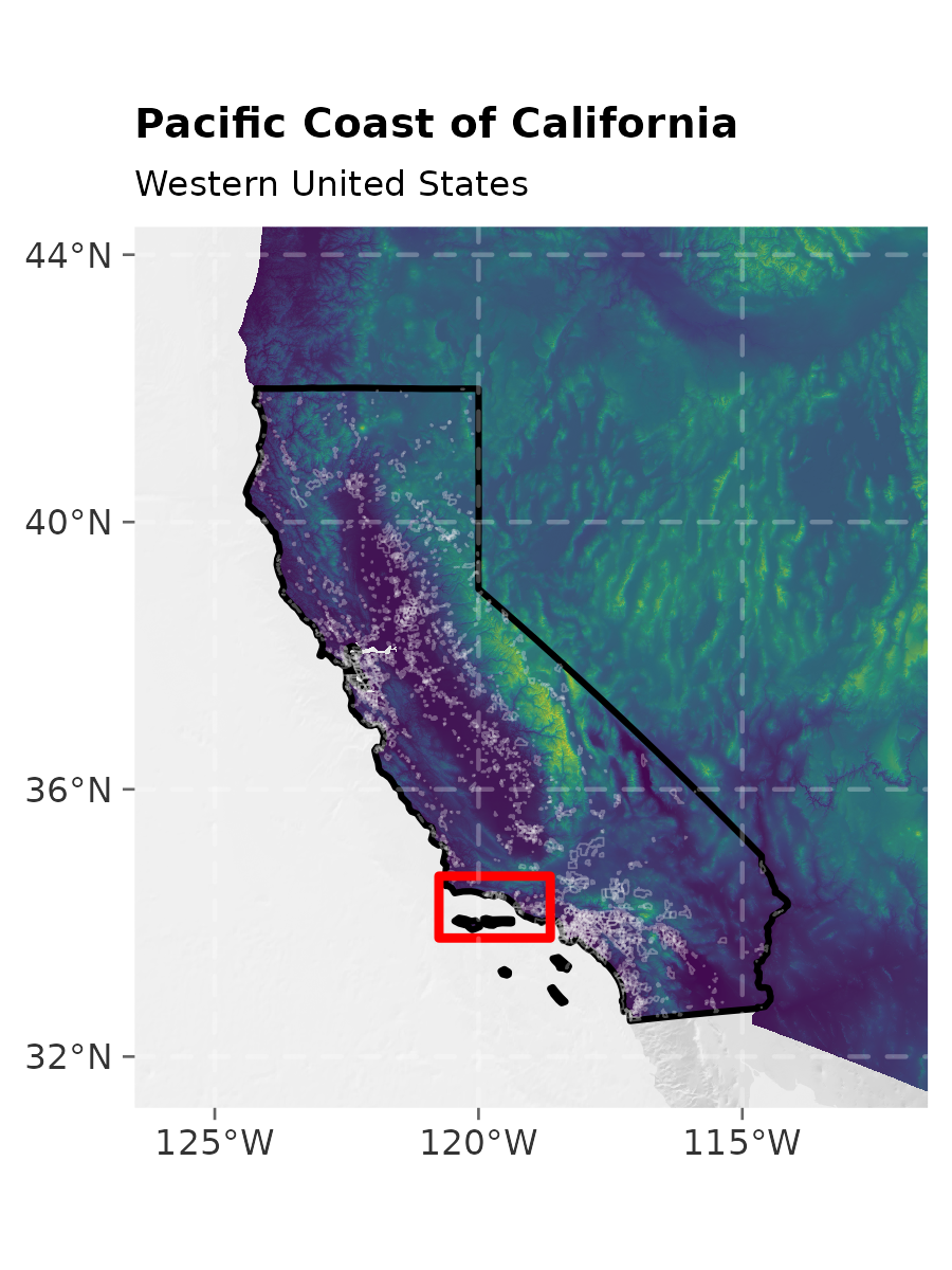
zoom_1_final_plot <- ggplot() +
  geom_raster(
    data = zoom_1_dem_df,
    aes(x = x, y = y, fill = dem90_hf)
  ) +
  scale_fill_viridis_c(guide = "none") +
  geom_raster(
    data = zoom_1_hillshade_df,
    aes(x = x, y = y, alpha = GRAY_HR_SR_OB)
  ) +
  scale_alpha(range = c(0.05, 0.3), guide = "none") +
  geom_spatvector(data = cal_poly, fill = NA, color = "black", linewidth = 0.7) +
  geom_spatvector(data = places_simple, fill = "NA", color = "#EEEEEE50", linewidth = 0.2) +
  geom_spatvector(data = zoom_2_crop_extent, color = "red", lwd = 1, fill = NA) +
  scale_x_continuous(breaks = seq(-125, -115, by = 5), labels = function(x) paste0(abs(x), "°W")) +
  scale_y_continuous(breaks = seq(32, 44, by = 4), labels = function(y) paste0(y, "°N")) +
  theme(
    plot.title = element_text(size = 9.5, face = "bold", hjust = 0.5),
    plot.subtitle = element_text(size = 8, hjust = 0.5),
    axis.title = element_blank(),
    axis.text = element_text(size = 8, color = "gray20"),
    axis.ticks = element_line(color = "gray40", linewidth = 0.3),
    legend.position = "none",
    panel.ontop = TRUE,
    panel.grid.major = element_line(color = "#FFFFFF44", linetype = "dashed"),
    panel.background = element_blank()
  ) +
  coord_sf(expand = FALSE) +
  labs(
    title = "Pacific Coast of California",
    subtitle = "Western United States"
  )

zoom_1_final_plot

#######################################################################################


ggsave("images/map3.png", width = 3, height = 4, plot = zoom_1_final_plot, bg = "white")
ggsave("final_output/map_03.png", width = 3, height = 4, plot = zoom_1_final_plot, bg = "white")