Map 11: Dibblee Geologic Map

Splicing adjacent quadrangles: Dos Pueblos Canyon (West) and Goleta (East)

Rendered Map Plates

Spliced Campus Geological Surface (Campus AOI)

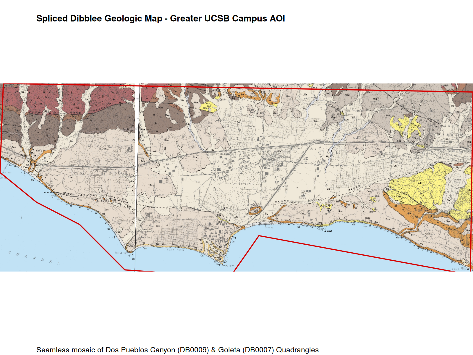
The finished atlas plate below shows the seamlessly spliced geological mosaic across the entire Greater UCSB Campus study area. The western section (North Campus Open Space, Devereux Slough, Coal Oil Point Reserve, and Ellwood) is sourced from the Dos Pueblos Canyon quadrangle, while the eastern section (Main Campus, Storke Campus, Goleta Slough, and Airport) is sourced from the Goleta quadrangle.

Map 11 Spliced Dibblee Map

Map 11: Spliced Dibblee geological map across the Greater UCSB Campus AOI

Intermediate Diagnostic: Full Extent of Both Sheets with Overlaid AOI

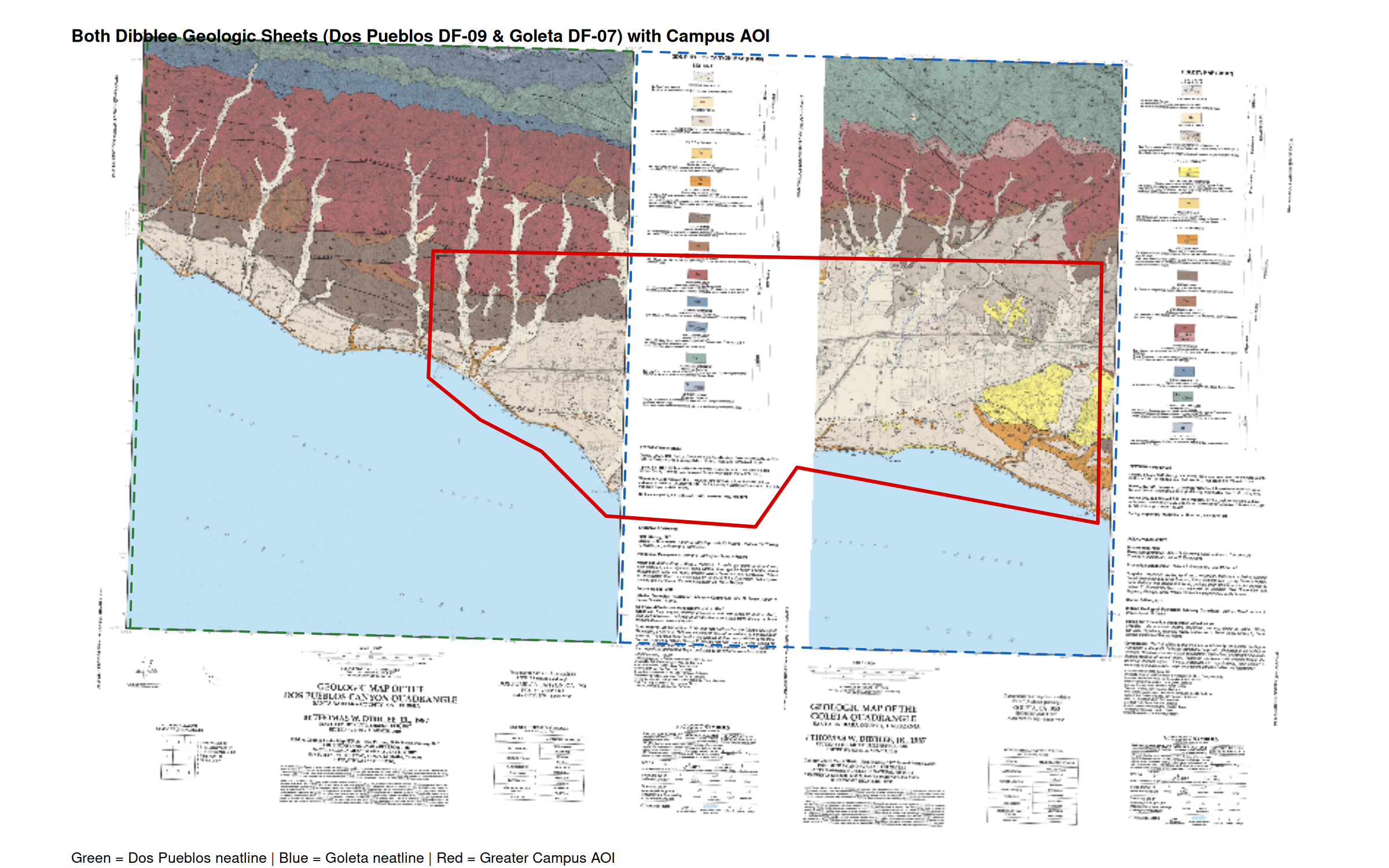
To visualize the spatial relationship between the two historic paper sheets and the campus study area, both uncropped, rectified sheets are displayed side by side:

Both Dibblee Sheets with AOI

Full Extent of Both Dibblee Sheets (Dos Pueblos DF-09 & Goleta DF-07) with Overlaid Campus AOI Boundary
NoteSpatial Splicing & The Dividing Meridian
  • Green dashed neatline: Dos Pueblos Canyon 7.5’ boundary (\(-120^\circ 00' 00''\) to \(-119^\circ 52' 30''\text{ W}\)).
  • Blue dashed neatline: Goleta 7.5’ boundary (\(-119^\circ 52' 30''\) to \(-119^\circ 45' 00''\text{ W}\)).
  • Red boundary: Greater UCSB Campus AOI (\(-119^\circ 55' 33''\) to \(-119^\circ 45' 15''\text{ W}\)).

The campus study area sits directly straddling the shared \(119^\circ 52' 30''\text{ W}\) dividing meridian. By trimming the paper collars to the neatline coordinates and merging them with terra::merge(), the two independent map sheets are spliced into a continuous geological continuum without white border artifacts.

An intermediate multi-sheet GeoTIFF is output to:
output_data/dibblee_both_tiffs_full_extent_with_aoi.tif (107 MB).


Standalone AOI Clip

Dibblee AOI Map

Dibblee AOI Clip

Technical Summary

  • Objective: Ingest two adjacent historic Dibblee geologic quadrangle sheets, rectify rotated affine grids into standard orthogonal space with terra::rectify(), trim paper collar margins to 7.5’ neatlines, splice the sheets into a continuous mosaic using terra::merge(), and clip the geological data to the Greater UCSB study area.
  • Key Packages: terra
  • Input Layers:
    • Western Sheet: Dos Pueblos Canyon 7.5’ Geologic Quadrangle (source_data/09gDosPueblos/DB0009.tif)
    • Eastern Sheet: Goleta 7.5’ Geologic Quadrangle (source_data/07gGoleta/DB0007.tif)
    • Campus Study Area: Greater UCSB Campus AOI (source_data/greater_UCSB-campus-aoi.geojson)
  • Generated Outputs:
    • Intermediate Full-Extent GeoTIFF: output_data/dibblee_both_tiffs_full_extent_with_aoi.tif
    • Diagnostic Overview Plate: images/map11_both_tiffs_full_extent_aoi.png & final_output/map11_both_tiffs_full_extent_aoi.png
    • Final Spliced Campus Plate: images/map11.png & final_output/map_11.png
    • Standalone Square Clip: final_output/dibble_aoi.png

Step-by-Step Cartographic Workflow & Intermediate Outputs

The script scripts/map_11.r details the end-to-end digital cartographic rectification, paper collar trimming, and mosaic splicing process.

Step 1: Affine Rectification of Scanned Historic Paper Maps

Historical scanned paper maps contain non-orthogonal scanner rotation and skew. Both DB0007.tif (Goleta) and DB0009.tif (Dos Pueblos Canyon) are rectified using bilinear interpolation into orthogonal coordinates (NAD27 / UTM zone 11N):

library(terra)

# Bilinear rectification to orthogonal UTM coordinates
gol <- rast("source_data/07gGoleta/DB0007.tif")
gol_rect <- rectify(gol, method = "bilinear")
names(gol_rect) <- c("red", "green", "blue")

dp <- rast("source_data/09gDosPueblos/DB0009.tif")
dp_rect <- rectify(dp, method = "bilinear")
names(dp_rect) <- c("red", "green", "blue")

Step 2: Intermediate Diagnostic — Full Uncropped Sheets with Neatlines and AOI

If the two raw map sheets were merged directly, the white paper collars, quadrangle titles, and bibliographic legends of one sheet would overwrite the geological data of the other. The script generates a diagnostic graphic displaying the uncropped sheets side-by-side with overlaid 7.5-minute neatlines and the campus AOI boundary:

# Intermediate diagnostic plot
png("final_output/map11_both_tiffs_full_extent_aoi.png", width = 2400, height = 1500, res = 150)
plotRGB(merge(aggregate(dp_rect, fact = 4), aggregate(gol_rect, fact = 4)))
plot(poly_dp, border = "#2E7D32", lwd = 2.5, lty = 2, add = TRUE) # Dos Pueblos neatline
plot(poly_gol, border = "#1565C0", lwd = 2.5, lty = 2, add = TRUE) # Goleta neatline
plot(aoi_nad27, border = "#D50000", lwd = 4, add = TRUE)            # Campus AOI
dev.off()

Map 11 Diagnostic Both Sheets

Intermediate Diagnostic: Both uncropped Dibblee sheets showing overlapping paper collars and the campus boundary

Step 3: Neatline Collar Trimming & Splicing Across the \(119^\circ 52' 30''\text{ W}\) Meridian

Both sheets are mathematically clipped to their official USGS 7.5-minute boundaries: * Dos Pueblos Canyon: \(-120.000^\circ\) to \(-119.875^\circ\text{ W}\) (East neatline at \(X = 235,715.5\text{ m}\)) * Goleta: \(-119.875^\circ\) to \(-119.750^\circ\text{ W}\) (West neatline at \(X = 235,715.5\text{ m}\))

By clipping exactly at \(X = 235,715.5\text{ m}\) in NAD27 / UTM zone 11N, terra::merge() seamlessly joins the two sheets without seamline artifacts or collar occlusion.

# Trim collars to shared neatline meridian and merge
poly_dp_aoi <- ext(222896, 235715.5, ymin(aoi_ext), ymax(aoi_ext))
poly_gol_aoi <- ext(235715.5, 252013, ymin(aoi_ext), ymax(aoi_ext))

dp_sub <- crop(dp_rect, poly_dp_aoi)
gol_sub <- crop(gol_rect, poly_gol_aoi)

spliced_campus <- merge(dp_sub, gol_sub)
campus_geology <- crop(spliced_campus, aoi_nad27)

Step 4: Standalone Campus AOI Crop

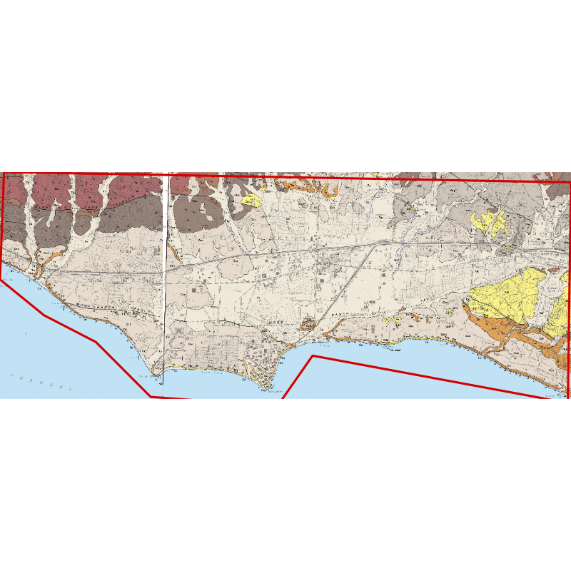
The spliced geological continuum is clipped to the Greater UCSB study area polygon and exported at high resolution.

Dibblee AOI Map

Intermediate Crop: Standalone campus geological clip

Full R Script (scripts/map_11.r)

Show R Code
# map 11
# Look at a Dibblee geologic map:
# Splicing two adjacent 7.5-minute quadrangles:
# West: Dos Pueblos Canyon (09gDosPueblos / DB0009.tif)
# East: Goleta (07gGoleta / DB0007.tif)

library(terra)

# Clean the environment and hidden objects
rm(list = ls())

# Set map number
current_sheet <- 11
# Set ggplot counter
current_ggplot <- 0

gg_labelmaker <- function(plot_num) {
  gg_title <- c("Map:", current_sheet, " ggplot:", plot_num)
  plot_text <- paste(gg_title, collapse = " ")
  print(plot_text)
  current_ggplot <<- plot_num
  return(plot_text)
}

# Ensure output directories exist
dir.create("images", showWarnings = FALSE)
dir.create("final_output", showWarnings = FALSE)
dir.create("output_data", showWarnings = FALSE)

crs_nad27 <- "+proj=utm +zone=11 +datum=NAD27 +units=m +no_defs"

# ---------- 1. Ingest & Rectify Both Dibblee Quadrangles ----------
# Goleta Quadrangle (DF-07 / DB0007.tif) - East side of campus
if (file.exists("output_data/DB0007_rectified.tif")) {
  cat("Loading cached rectified Goleta quadrangle (DB0007)...\n")
  gol_rect <- rast("output_data/DB0007_rectified.tif")
} else {
  cat("Rectifying Goleta quadrangle (DB0007)...\n")
  gol <- rast("source_data/07gGoleta/DB0007.tif")
  gol_rect <- rectify(gol, method = "bilinear")
  names(gol_rect) <- c("red", "green", "blue")
  writeRaster(gol_rect, "output_data/DB0007_rectified.tif", overwrite = TRUE, gdal = c("COMPRESS=DEFLATE", "TILED=YES"))
}

# Dos Pueblos Canyon Quadrangle (DF-09 / DB0009.tif) - West side of campus
dp_file <- "source_data/09gDosPueblos/DB0009.tif"
if (!file.exists(dp_file)) {
  # Check alternate location if applicable
  dp_file <- "source_data/16gSolvangGaviota/DB0016.tif"
}

if (file.exists("output_data/DB0009_rectified.tif")) {
  cat("Loading cached rectified Dos Pueblos Canyon quadrangle (DB0009)...\n")
  dp_rect <- rast("output_data/DB0009_rectified.tif")
} else if (file.exists(dp_file)) {
  cat("Rectifying Dos Pueblos Canyon quadrangle (DB0009)...\n")
  dp <- rast(dp_file)
  dp_rect <- rectify(dp, method = "bilinear")
  names(dp_rect) <- c("red", "green", "blue")
  writeRaster(dp_rect, "output_data/DB0009_rectified.tif", overwrite = TRUE, gdal = c("COMPRESS=DEFLATE", "TILED=YES"))
} else {
  stop("Western Dibblee quadrangle not found! Please place DB0009.tif in source_data/09gDosPueblos/")
}

# ---------- 2. Campus AOI and Quadrangle Neatlines ----------
aoi <- vect("source_data/greater_UCSB-campus-aoi.geojson")
aoi_nad27 <- project(aoi, crs_nad27)

# Goleta 7.5' neatline: -119.875° to -119.750° W, 34.375° to 34.500° N
poly_gol <- project(as.polygons(ext(-119.875, -119.750, 34.375, 34.500), crs = "EPSG:4326"), crs_nad27)

# Dos Pueblos Canyon 7.5' neatline: -120.000° to -119.875° W, 34.375° to 34.500° N
poly_dp <- project(as.polygons(ext(-120.000, -119.875, 34.375, 34.500), crs = "EPSG:4326"), crs_nad27)

# ---------- 3. Output Intermediate GeoTIFF of Both Full Sheets with AOI ----------
interm_tif <- "output_data/dibblee_both_tiffs_full_extent_with_aoi.tif"
if (!file.exists(interm_tif)) {
  cat("Generating intermediate GeoTIFF showing full extent of both sheets with AOI...\n")
  dp_half <- aggregate(dp_rect, fact = 2)
  gol_half <- aggregate(gol_rect, fact = 2)
  both_full <- merge(dp_half, gol_half)

  aoi_buf <- buffer(as.lines(aoi_nad27), width = 60)
  both_with_aoi <- rasterize(aoi_buf, both_full, update = TRUE)

  writeRaster(both_with_aoi, interm_tif, overwrite = TRUE, gdal = c("COMPRESS=DEFLATE", "TILED=YES"))
}

# Diagnostic overview PNG showing full extent of both sheets + neatlines + AOI:
png("final_output/map11_both_tiffs_full_extent_aoi.png", width = 2400, height = 1500, res = 150)
plotRGB(merge(aggregate(dp_rect, fact = 4), aggregate(gol_rect, fact = 4)))
plot(poly_dp, border = "#2E7D32", lwd = 2.5, lty = 2, add = TRUE)
plot(poly_gol, border = "#1565C0", lwd = 2.5, lty = 2, add = TRUE)
plot(aoi_nad27, border = "#D50000", lwd = 4, add = TRUE)
title(
  main = "Both Dibblee Geologic Sheets (Dos Pueblos DF-09 & Goleta DF-07) with Campus AOI",
  sub = "Green = Dos Pueblos neatline | Blue = Goleta neatline | Red = Greater Campus AOI"
)
dev.off()
file.copy("final_output/map11_both_tiffs_full_extent_aoi.png", "images/map11_both_tiffs_full_extent_aoi.png", overwrite = TRUE)

# ---------- 4. Splicing the 2 Maps Together (Neatline Collar-Trimmed) ----------
cat("Trimming collars to neatlines and splicing adjacent sheets...\n")
# Bounding extent covering the AOI latitude range:
aoi_ext <- ext(aoi_nad27) + c(-200, 200, -200, 200)

poly_dp_aoi <- ext(222896, 235715.5, ymin(aoi_ext), ymax(aoi_ext))
poly_gol_aoi <- ext(235715.5, 252013, ymin(aoi_ext), ymax(aoi_ext))

dp_sub <- crop(dp_rect, poly_dp_aoi)
gol_sub <- crop(gol_rect, poly_gol_aoi)

spliced_campus <- merge(dp_sub, gol_sub)

# Crop spliced mosaic to the Greater Campus AOI:
campus_geology <- crop(spliced_campus, aoi_nad27)

# ---------- 5. Save Final Spliced Map Outputs ----------
png("images/map11.png", width = 1600, height = 1200, res = 150)
plotRGB(campus_geology)
plot(aoi_nad27, border = "#D50000", lwd = 2.5, add = TRUE)
title(
  main = "Spliced Dibblee Geologic Map - Greater UCSB Campus AOI",
  sub = "Seamless mosaic of Dos Pueblos Canyon (DB0009) & Goleta (DB0007) Quadrangles"
)
dev.off()
file.copy("images/map11.png", "final_output/map_11.png", overwrite = TRUE)

# Also save standalone AOI clip
png("final_output/dibble_aoi.png", width = 800, height = 800, res = 150)
plotRGB(campus_geology)
plot(aoi_nad27, border = "#D50000", lwd = 2, add = TRUE)
dev.off()

cat("\nMap 11 successfully generated:\n")
cat(" - Intermediate GeoTIFF: output_data/dibblee_both_tiffs_full_extent_with_aoi.tif\n")
cat(" - Diagnostic Full Map:  final_output/map11_both_tiffs_full_extent_aoi.png\n")
cat(" - Final Spliced Plate:  final_output/map_11.png\n")
cat(" - Square AOI Clip:      final_output/dibble_aoi.png\n")