# map 2
# Stylized trees, bikeways, walkways, and water

## Two water sources used until now:
##  * Pacific Ocean Polygon https://geodata.library.ucsb.edu/catalog/3853-s3_2002_s3_reg_pacific_ocean
##  * California Streams https://data.cnra.ca.gov/dataset/california-streams
# core skills from the lesson are in ep. 7

# clean the environment and hidden objects
rm(list = ls())

# make our ggtitles automagically #######
# set map number
current_sheet <- 2
# set ggplot counter
current_ggplot <- 0

gg_labelmaker <- function(plot_num) {
  gg_title <- c("Map:", current_sheet, " ggplot:", plot_num)
  plot_text <- paste(gg_title, collapse = " ")
  print(plot_text)
  current_ggplot <<- plot_num
  return(plot_text)
}
# every ggtitle should be:
# ggtitle(gg_labelmaker(current_ggplot+1))
# end automagic ggtitle           #######


# Load required libraries
library(tidyverse)
library(terra) # Required for loading vector data with vect() function
library(tidyterra) # Required for using geom_spatvector() with ggplot
library(ggspatial) # Required for map scale -annotation_scale()- and compass -annotation_north_arrow()-
library(ggnewscale) # Required for mapping multiple scales in ggplot
library(sf)


## Read data
# Trees
trees <- vect("source_data/Treekeeper_012116/DTK_012116.shp")
# Bikes
bikes <- vect("source_data/icm_bikes/bike_paths/bikelanescollapsedv8.shp")
# Streams
streams <- vect("source_data/california_streams/California_Streams.shp")
# Coastline polygon
coastline <- vect("source_data/pacific_ocean-shapefile/3853-s3_2002_s3_reg_pacific_ocean_lines.shp")
# IV buildings
iv_buildings <- st_read("source_data/iv_buildings/iv_buildings/CA_Structures_ExportFeatures.shp")
# NCOS multi-use trails
ncos_trails <- vect("source_data/ncos_trails/ncos_multiuse_trails.geojson")

# Let's take a quick first look at our data and find out their projections
plot(trees)
crs(trees, describe = TRUE)
plot(bikes)
crs(bikes, describe = TRUE)

# this streams is giant.
# plot(streams)
crs(streams, describe = TRUE)
# plot(coastline)
# plot(streams)
# crs(streams, describe=TRUE)
plot(coastline)
crs(coastline, describe = TRUE)

# 3 different CRSs at least:
# * Trees: WGS84 - Pseudo-mercator / EPSG 3857
# * Bikes: NAD83 / EPSG 2229
# * Streams: WGS84  - Pseudo-mercator / EPSG 3857
# * Coastline: WGS84 / EPSG 4326

# So our first step will be to reproject our data to a common CRS. As the most
# common one is WGS84 - Pseudo-mercator / EPSG 3857 from the `trees` and `streams`
# data, we will use that one

# Use the project() function, the first parameter is the SpatVector we want to
# reproject, and the second argument is the desired crs we want it reprojected to.
# For the second argument, we can supply a SpatVector and terra will automatically
# get the crs from that SpatVector
bikes_proj <- project(bikes, trees)
coastline_proj <- project(coastline, trees)
ncos_proj <- project(ncos_trails, trees)


## Challenge: Do we need to reproject the streams data?

# Now that our data is in the same CRS, let's check their extent
ext(trees)
# * SpatExtent : -13344813.2450353, -13340270.0860384, 4083607.02801381, 4085810.69483412 (xmin, xmax, ymin, ymax)

ext(streams)
# * SpatExtent : -13851388.1259, -12638118.6176, 3827948.8521, 5309358.2157 (xmin, xmax, ymin, ymax)

ext(bikes_proj)
# * SpatExtent : -13344859.3101604, -13340139.1335369, 4083614.50498653, 4085816.84965297 (xmin, xmax, ymin, ymax)

ext(coastline_proj)
# * SpatExtent : -13358945.2438268, -13336909.6752497, 4074087.46157742, 4090166.00468701 (xmin, xmax, ymin, ymax)


# Our data has very different extents, as the trees and bikes data covers only campus,
# and the coastline and streams data cover all of California. For
# this reason, we will use the terra:crop() function so all SpatVectors have the
# same extent.

# We will base our map in the extent of the `trees` data, so we will crop all vectors
# to the extent of the `trees` data
bikes_crop <- crop(bikes_proj, trees)
streams_crop <- crop(streams, trees)
coastline_crop <- crop(coastline_proj, trees)


# With these datasets, let's do a first test of how our map would look like
ggplot() +
  geom_spatvector(data = trees, colour = "green4") +
  geom_spatvector(data = streams_crop, colour = "lightblue") +
  geom_spatvector(data = bikes_crop, colour = "black") +
  geom_spatvector(data = coastline_crop, colour = "darkblue") +
  geom_spatvector(data = iv_buildings) +
  ggtitle(gg_labelmaker(current_ggplot + 1)) +
  coord_sf()


# But we see that the current extent used is too narrow, we almost can't see
# the water streams or the offshore contours. So we are going to zoom out
# a 25% of the range in the x and y axis

# Store extent as object called `ext_trees`
ext_trees <- ext(trees)
# Calculate range in each axis
xrange <- ext_trees$xmax - ext_trees$xmin
yrange <- ext_trees$ymax - ext_trees$ymin
# Increase range by 25%
xrange <- xrange * 0.25
yrange <- yrange * 0.25
# Create new extent
new_ext <- ext(
  -xrange + ext_trees$xmin, xrange + ext_trees$xmax,
  -yrange + ext_trees$ymin, yrange + ext_trees$ymax
)

# Crop the SpatVectors again, but with the new extent
bikes_crop <- crop(bikes_proj, new_ext)
streams_crop <- crop(streams, new_ext)
coastline_crop <- crop(coastline_proj, new_ext)
ncos_crop <- crop(ncos_proj, new_ext)
iv_crop_poly <- st_as_sf(as.polygons(new_ext))
# iv_buildings <- st_crop(iv_buildings, iv_crop_poly)

# Run again the plot to see the differences
ggplot() +
  geom_spatvector(data = trees, colour = "green4") +
  geom_spatvector(data = streams_crop, , colour = "lightblue") +
  geom_spatvector(data = bikes_crop, colour = "black") +
  geom_spatvector(data = coastline_crop, colour = "darkblue") +
  geom_spatvector(data = iv_buildings) +
  ggtitle(gg_labelmaker(current_ggplot + 1)) +
  coord_sf()

# We will come back to stylize our map even more, but for now, let's explore
# the trees data, which contains more information beyond points for the location
# of the trees

# Let's see the names of the columns included in the trees data and some values of each
names(trees)
summary(trees)
head(trees)

# We can see a number of interesting features included in the data, like the
# location (Geogx, STREET and ADDRESS attributes), species (SPP), height (HT),
# condition (COND)
unique(trees$SPP)
summary(trees$HT)

# Let's plot the trees data scaling each point according to the height of the tree
ggplot() +
  geom_spatvector(data = trees, aes(size = HT), colour = "green4") +
  ggtitle(gg_labelmaker(current_ggplot + 1), subtitle = "Tree Heights")

# We could modify it a bit to reduce the scale of the dots. Here the values
# in the range parameter means the size in milimeters of the dots, going from
# 0 mm to 2 mm
ggplot() +
  geom_spatvector(data = trees, aes(size = HT), colour = "green4") +
  scale_size_continuous(range = c(0, 2)) +
  ggtitle(gg_labelmaker(current_ggplot + 1), subtitle = "Tree Heights")


# But we can notice that there are trees with height 0, seedlings. Do we want to
# keep these? Probably not. We could make a histogram to see the distribution
# of the heights of the trees. But instead, let's just print the percentage of
# trees (or which is the same, the percentage of rows in the dataset) with
# height 0
ht_0 <- trees %>%
  filter(HT == 0) %>%
  nrow()
total <- nrow(trees)
perc_0 <- (ht_0 / total) * 100
print(sprintf("%.2f%%", perc_0))

# So we are going to filter our the 1,480 observations (13.46% of the total) of
# trees with height 0
trees_filt <- trees %>%
  filter(HT > 0)

# Let's plot again to see the difference
ggplot() +
  geom_spatvector(data = trees_filt, aes(size = HT), colour = "green4") +
  scale_size_continuous(range = c(0, 2))

# Now we can starting adding our other sets of data. To start with, the water streams,
# changing the theme to minimal
ggplot() +
  geom_spatvector(data = trees_filt, aes(size = HT), colour = "green4") +
  scale_size_continuous(range = c(0, 2)) +
  geom_spatvector(data = streams_crop, colour = "cadetblue3") +
  theme_minimal()

# Increasing the width of the lines that represent the streams and including
# it in the legend
ggplot() +
  geom_spatvector(data = trees_filt, aes(size = HT, colour = "Trees"), alpha = 0.5) +
  scale_size_continuous(range = c(0, 2), name = "Tree Height (ft)") +
  geom_spatvector(data = streams_crop, aes(colour = "Streams"), linewidth = 2, alpha = 0.6) +
  scale_colour_manual(
    name = "Legend",
    values = c(
      "Trees" = "green4",
      "Streams" = "cadetblue3"
    )
  ) +
  ggtitle(gg_labelmaker(current_ggplot + 1)) +
  theme_minimal()


## Challenge: What is the difference between setting the color of the trees
#   inside the aes of the geom_spatvector layer and inside the scale_color_manual
#   layer?

# Including the bike paths
ggplot() +
  geom_spatvector(data = trees_filt, aes(size = HT, colour = "Trees"), alpha = 0.5) +
  scale_size_continuous(range = c(0, 2), name = "Tree Height (ft)") +
  geom_spatvector(data = streams_crop, aes(colour = "Streams"), , linewidth = 2, alpha = 0.6) +
  geom_spatvector(data = bikes_crop, aes(colour = "Bike Paths"), linewidth = 1) +
  scale_colour_manual(
    name = "Legend",
    values = c(
      "Trees" = "green4",
      "Streams" = "cadetblue3",
      "Bike Paths" = "black"
    )
  ) +
  theme_minimal()

# We can notice a problem here, as in the legend the bike paths seem to be a
# polygon and not a line

# If we transform this data to a data frame, we can see that it only contains
# 4 rows, and the first of this is a MULTILINESTRING, which potentially is
# causing our legend to not display correctly as a line. If you also transform
# streams_crop as a data frame, you'll notice that each geometry is a LINESTRING
# which makes it plot correctly in the legend
biked_df <- as.data.frame(bikes_crop, geom = "WKT")
biked_df

# To fix this, we need to dissagregate the MULTILINESTRING of bike paths into
# individual LINESTRINGs. For that, we can use the `disagg` terra function, which
# separates multi-objects into single objects
bikes_lines <- disagg(bikes_crop)
ncos_lines <- disagg(ncos_crop)

# Trying again the same plot to check the differences
ggplot() +
  geom_spatvector(data = trees_filt, aes(size = HT, colour = "Trees"), alpha = 0.5) +
  scale_size_continuous(range = c(0, 2), name = "Tree Height (ft)") +
  geom_spatvector(data = streams_crop, aes(colour = "Streams"), , linewidth = 2, alpha = 0.4) +
  geom_spatvector(data = bikes_lines, aes(colour = "Bike Paths"), linewidth = 1) +
  scale_colour_manual(
    name = "Legend",
    values = c(
      "Trees" = "green4",
      "Streams" = "cadetblue3",
      "Bike Paths" = "black"
    )
  ) +
  theme_minimal()

# Finally adding the coastline geometry and legend.
# Save this plot in an object so we don't have to repeat the same code
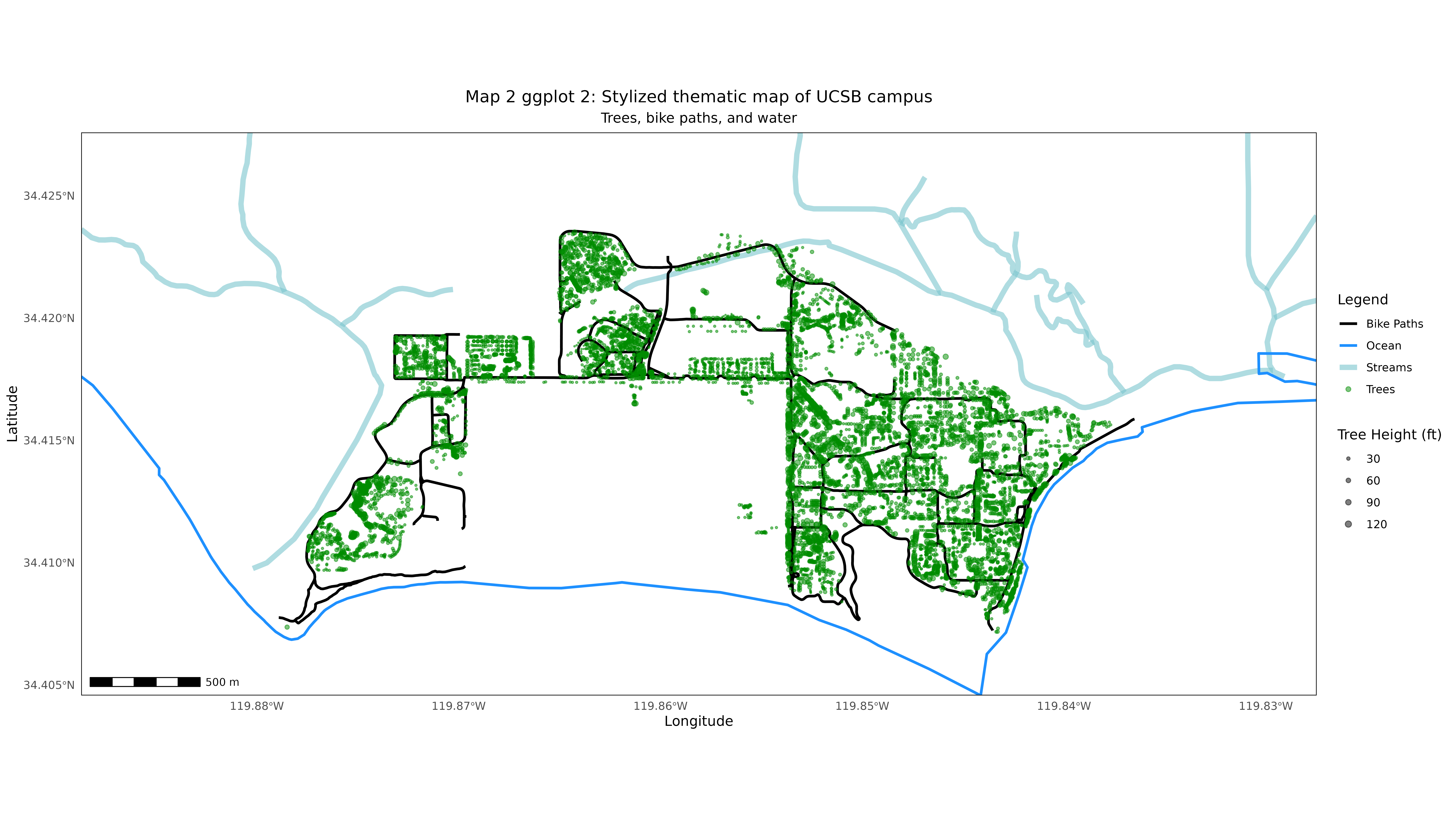
map2_gg1 <- ggplot() +
  geom_spatvector(data = streams_crop, aes(colour = "Streams"), , linewidth = 2, alpha = 0.6) +
  geom_spatvector(data = bikes_lines, aes(colour = "Bike Paths"), linewidth = 1) +
  geom_spatvector(data = trees_filt, aes(size = HT, colour = "Trees"), alpha = 0.5) +
  scale_size_continuous(range = c(0, 2), name = "Tree Height (ft)") +
  geom_spatvector(data = coastline_crop, aes(colour = "Ocean"), linewidth = 1, fill = "dodgerblue") +
  scale_colour_manual(
    name = "Legend",
    values = c(
      "Trees" = "green4",
      "Bike Paths" = "black",
      "Streams" = "cadetblue3",
      "Ocean" = "dodgerblue"
    )
  ) +
  theme_minimal()
map2_gg1

# Adding title, subtitle and title for the axes
map2_gg2 <- map2_gg1 +
  labs(
    title = "Map 2 ggplot 2: Stylized thematic map of UCSB campus",
    subtitle = "Trees, bike paths, and water",
    x = "Longitude", y = "Latitude"
  )
map2_gg2


# Modifying the aesthetics of the title and subtitle, removing the grid lines,
# and adding a black border around the map
# title and subtitle. Additionally, eliminating the white space between the
# plot region and the border
map2_gg3 <- map2_gg2 +
  theme(
    plot.title = element_text(hjust = 0.5),
    plot.subtitle = element_text(hjust = 0.5),
    panel.grid = element_blank(),
    panel.border = element_rect(color = "black", fill = NA, linewidth = 0.5)
  ) +
  scale_x_continuous(expand = c(0, 0)) +
  scale_y_continuous(expand = c(0, 0))
map2_gg3

# Finally, adding a scale
map2_gg4 <- map2_gg3 +
  annotation_scale(location = "bl", width_hint = 0.1)
map2_gg4

# Save this plot
ggsave(
  "images/map2_TreeHeight.png",
  plot = map2_gg4,
  width = 16, height = 9,
  dpi = 500,
  units = "in",
  bg = "white"
)

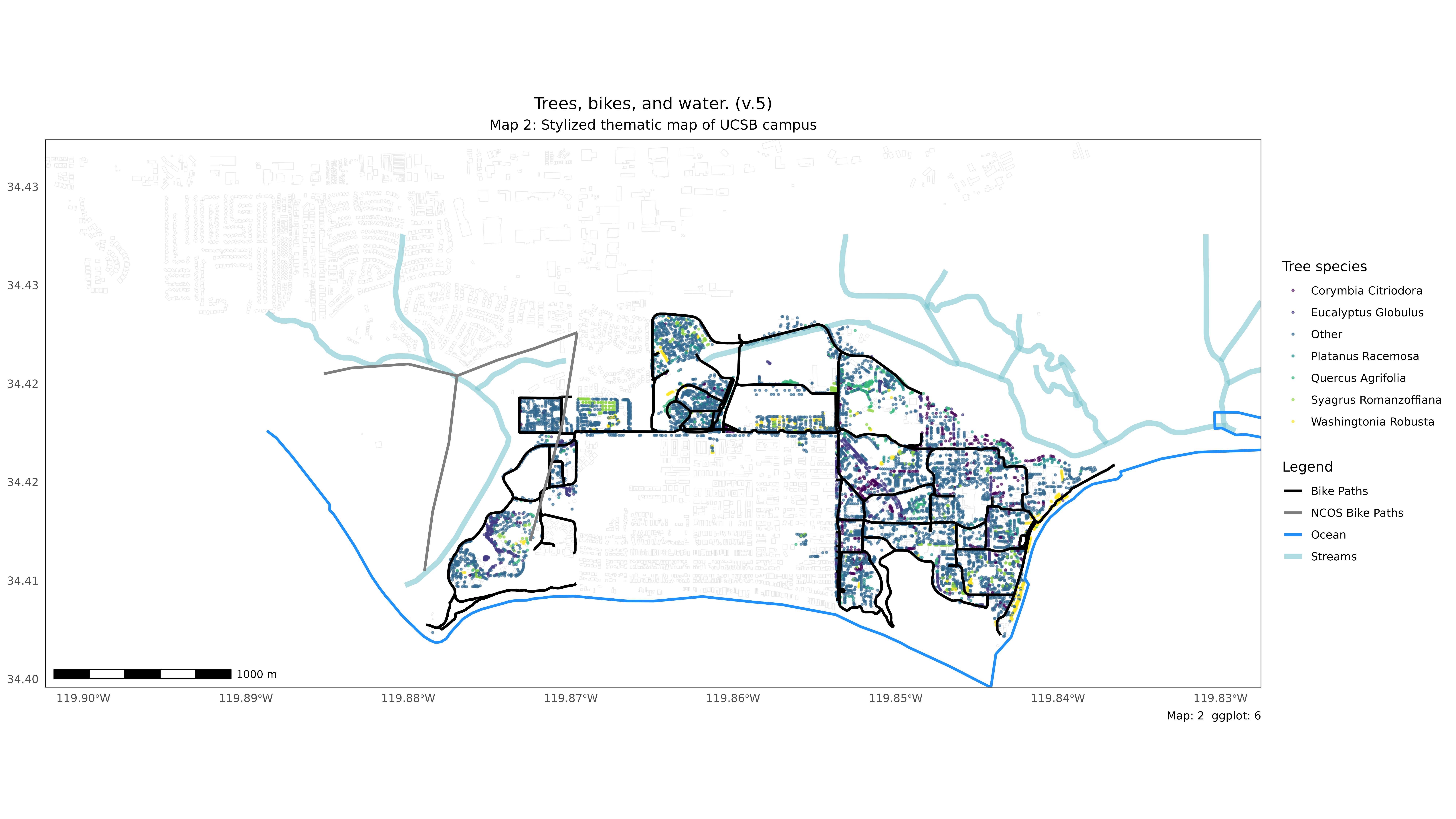
# We could make a different version of the plot, where we color the trees by their
# species

# We can see that there are 245 unique species of trees in our trees_filt data set
unique(trees_filt$SPP)

# For this reason, we are going to only color the 5 more frequent and leave all
# other species grouped in a category called 'Other'

# From our data, we count the frequencies over the SPP (species) attribute,
# then we return the top 5 with the head() function, and then we pull
# only the species names with the pull() function.
top5_species <- trees_filt %>%
  count(SPP, sort = TRUE) %>%
  head() %>%
  pull(SPP)

# Assign the same value (name) of the species if it is in the top5_species vector
# or 'Other if it's not. The result is assigned to a new attribute of our
# SpatVector called SPP_grouped
trees_filt$SPP_grouped <- ifelse(trees_filt$SPP %in% top5_species,
  str_to_title(trees_filt$SPP),
  "Other"
)

# Finally, making the plot with the same aesthetics as the previous one
map2_gg5 <- ggplot() +
  geom_spatvector(data = trees_filt, aes(colour = SPP_grouped), alpha = 0.6, size = 0.5) +
  scale_color_viridis_d(name = "Tree species") +
  new_scale_color() +
  geom_spatvector(data = streams_crop, aes(colour = "Streams"), , linewidth = 2, alpha = 0.6) +
  geom_spatvector(data = bikes_lines, aes(colour = "Bike Paths"), linewidth = 1) +
  geom_spatvector(data = ncos_lines, aes(colour = "NCOS Bike Paths"), linewidth = 1) +
  geom_spatvector(data = coastline_crop, aes(colour = "Ocean"), linewidth = 1, fill = "dodgerblue") +
  geom_sf(data = iv_buildings, color = alpha("gray60", 0.2), fill = NA) +
  scale_colour_manual(
    name = "Legend",
    values = c(
      "Bike Paths" = "black",
      "NCOS Bike Paths" = "gray50",
      "Streams" = "cadetblue3",
      "Ocean" = "dodgerblue"
    )
  ) +
  theme_minimal() +
  labs(
    subtitle = "Map 2: Stylized thematic map of UCSB campus",
    title = "Trees, bikes, and water. (v.5)",
    caption = gg_labelmaker(current_ggplot + 1),
    x = NULL, y = NULL
  ) +
  theme(
    plot.title = element_text(hjust = 0.5),
    plot.subtitle = element_text(hjust = 0.5),
    panel.grid = element_blank(),
    panel.border = element_rect(color = "black", fill = NA, linewidth = 0.5)
  ) +
  scale_x_continuous(expand = c(0, 0)) +
  scale_y_continuous(expand = c(0, 0), labels = scales::label_number(accuracy = 0.01)) +
  annotation_scale(location = "bl", width_hint = 0.167)
map2_gg5

# Save this plot
ggsave(
  "images/map2_5_TreeSpecies.png",
  plot = map2_gg5,
  width = 16, height = 9,
  dpi = 500,
  units = "in",
  bg = "white"
)

ggsave(
  "readme_images/map2_TreeSpecies.png",
  plot = map2_gg5,
  width = 16, height = 9,
  dpi = 500,
  units = "in",
  bg = "white"
)


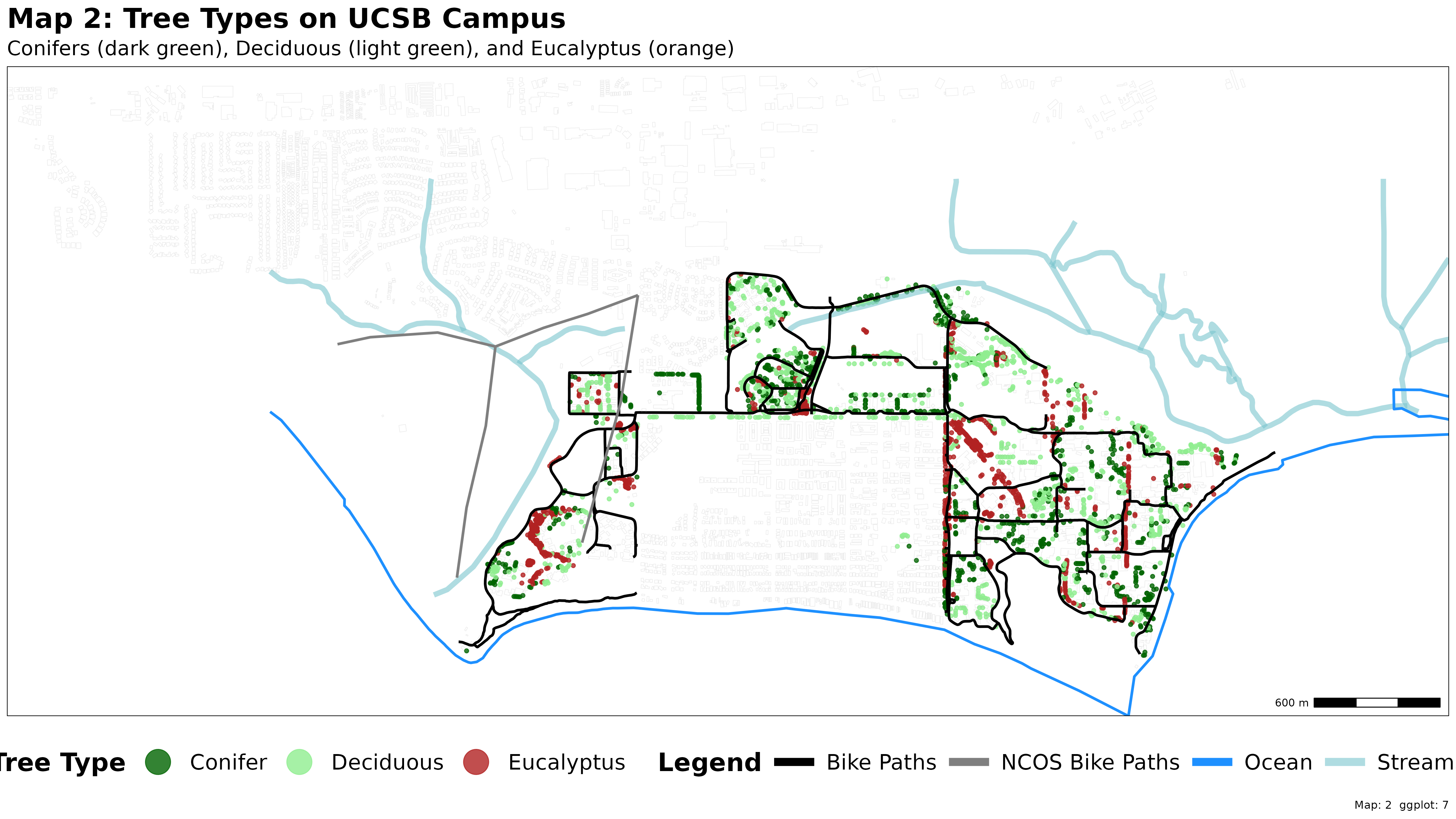
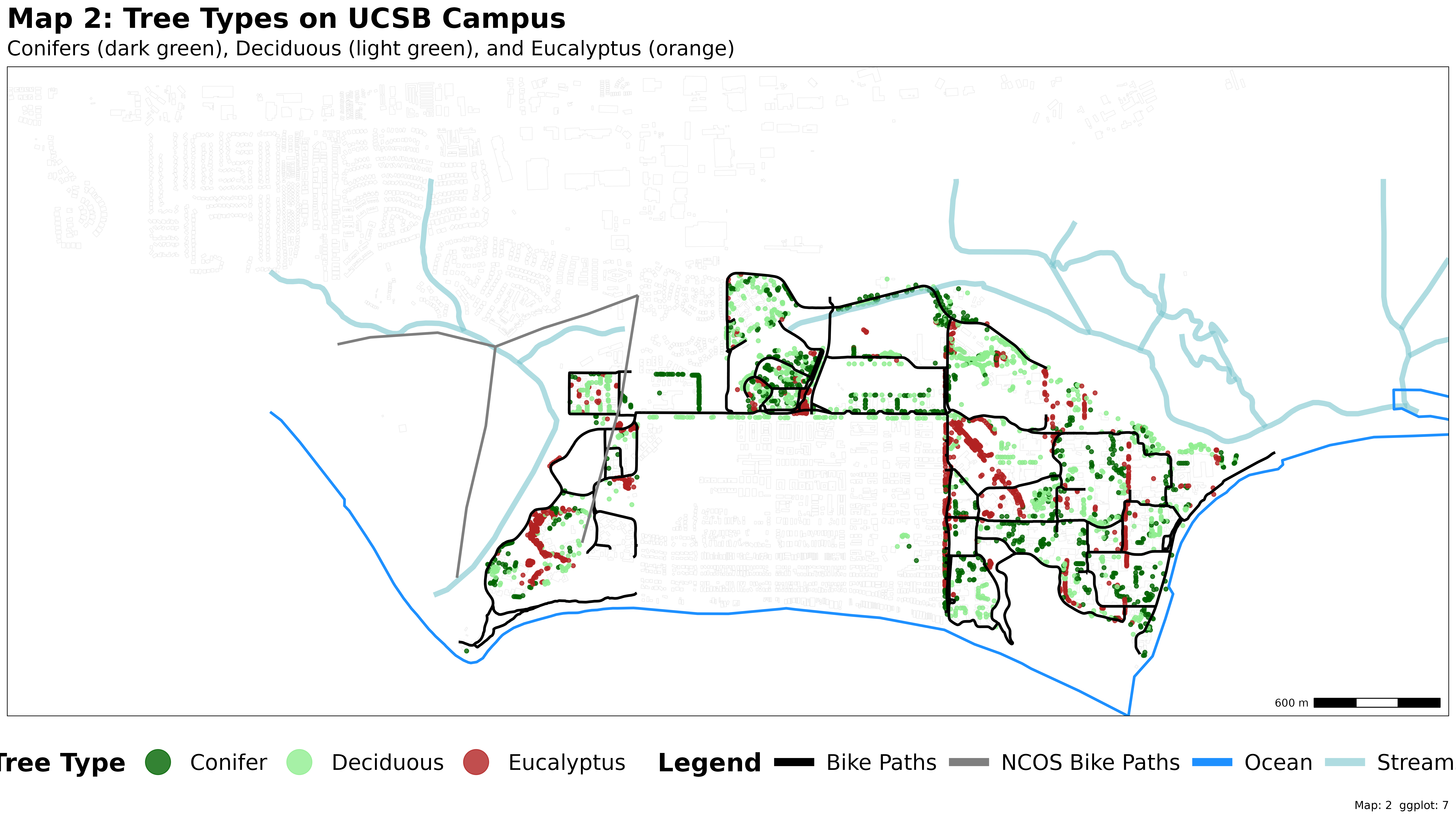
# Group trees by type: Conifer, Deciduous, Eucalyptus
# Using str_detect from stringr (part of tidyverse) to find keywords in species names
trees_filt$Tree_Type <- case_when(
  str_detect(trees_filt$SPP, regex("PINUS|CEDRUS|CUPRESSUS|SEQUOIA|PICEA|ABIES", ignore_case = TRUE)) ~ "Conifer",
  str_detect(trees_filt$SPP, regex("QUERCUS|PLATANUS|ACER|ALNUS|BETULA|FAGUS|SALIX|POPULUS|PRUNUS", ignore_case = TRUE)) ~ "Deciduous",
  str_detect(trees_filt$SPP, regex("EUCALYPTUS", ignore_case = TRUE)) ~ "Eucalyptus",
  TRUE ~ "Other"
)

summary(trees_filt)
names(trees_filt)
unique(trees_filt$Tree_Type)

tree_colors <- c(
  "Conifer" = "darkgreen",
  "Deciduous" = "lightgreen",
  "Eucalyptus" = "firebrick"
)

trees_filt$Tree_Type != "Other"

# Create a new plot coloring trees by their general type
map2_gg6 <- ggplot() +
  # Plot only the categorized trees, leave "Other" out for clarity
  geom_spatvector(data = subset(trees_filt, trees_filt$Tree_Type != "Other"), aes(colour = Tree_Type), alpha = 0.8, size = 1.2) +
  scale_colour_manual(
    name = "Tree Type",
    values = tree_colors,
    guide = guide_legend(override.aes = list(size = 9), order = 1)
  ) +
  new_scale_color() + # Reset color scale for the layers below
  geom_spatvector(data = streams_crop, aes(colour = "Streams"), linewidth = 2, alpha = 0.6) +
  geom_spatvector(data = bikes_lines, aes(colour = "Bike Paths"), linewidth = 1) +
  geom_spatvector(data = ncos_lines, aes(colour = "NCOS Bike Paths"), linewidth = 1) +
  geom_spatvector(data = coastline_crop, aes(colour = "Ocean"), linewidth = 1, fill = "dodgerblue") +
  geom_sf(data = iv_buildings, color = alpha("gray60", 0.2), fill = NA) +
  scale_colour_manual(
    name = "Legend",
    values = c(
      "Bike Paths" = "black",
      "NCOS Bike Paths" = "gray50",
      "Streams" = "cadetblue3",
      "Ocean" = "dodgerblue"
    ),
    guide = guide_legend(override.aes = list(linewidth = 3), order = 2)
  ) +
  theme_minimal() +
  labs(
    title = "Map 2: Tree Types on UCSB Campus",
    subtitle = "Conifers (dark green), Deciduous (light green), and Eucalyptus (orange)",
    caption = gg_labelmaker(current_ggplot + 1),
    x = NULL, y = NULL
  ) +
  theme(
    plot.title = element_text(hjust = 0.5, size = 22, face = "bold"),
    plot.subtitle = element_text(hjust = 0.5, size = 16),
    axis.title = element_blank(),
    axis.text = element_blank(),
    axis.ticks = element_blank(),
    panel.grid = element_blank(),
    panel.border = element_rect(color = "black", fill = NA, linewidth = 0.5),
    legend.position = "bottom",
    legend.box = "horizontal",
    legend.title = element_text(size = 20, face = "bold"),
    legend.text = element_text(size = 17),
    legend.key.size = unit(1.4, "cm"),
    legend.spacing.x = unit(0.5, "cm")
  ) +
  scale_x_continuous(expand = c(0, 0)) +
  scale_y_continuous(expand = c(0, 0)) +
  annotation_scale(location = "br", width_hint = 0.1)

map2_gg6

# Save the new plot
ggsave(
  "images/map2_TreeTypes.png",
  plot = map2_gg6,
  width = 16, height = 9,
  dpi = 500,
  units = "in",
  bg = "white"
)
ggsave("final_output/map_02.png", width = 16, height = 9, plot = map2_gg6, bg = "white")