#################################################
# zoom3
# Map 5 ########################################
#

# clean the environment and hidden objects

rm(list=ls())

library(sf)
library(terra)
library(tidyterra)
library(geojsonsf)
library(ggplot2)
library(dplyr)

# set map number
current_sheet <- 5
# set ggplot counter
current_ggplot <- 0

# our auto ggtitle maker
gg_labelmaker <- function(plot_num){
  gg_title <- c("Map:", current_sheet, " ggplot:", plot_num)
  plot_text <- paste(gg_title, collapse=" " )
  print(plot_text)
  current_ggplot <<- plot_num
  return(plot_text)
}
# every ggtitle should be:
# ggtitle(gg_labelmaker(current_ggplot+1))
# end automagic ggtitle


# ###########################
# Map 5
# Zoom 3: UCSB & Environs
# these come pre-made

campus_DEM <- rast("source_data/campus_DEM.tif")
plot(campus_DEM)
png("images/map5_base_dem.png", width = 1200, height = 900, res = 300)
plot(campus_DEM)
dev.off()

zoom_3_hillshade <- rast("source_data/campus_hillshade.tif")
plot(zoom_3_hillshade)
png("images/map5_base_hillshade.png", width = 1200, height = 900, res = 300)
plot(zoom_3_hillshade)
dev.off()


#################################################
# zoom3 as ggplot
campus_hillshade <- rast("source_data/campus_hillshade.tif")
str(campus_hillshade)
zoom_3_hillshade_df <- as.data.frame(campus_hillshade, xy=TRUE)
colnames(zoom_3_hillshade_df)

# let's make our ggplots shorter by saving
# our theme:
my_theme <- theme_minimal() +
  theme(axis.title.x = element_blank(),
        axis.title.y = element_blank(),
        axis.text.x = element_blank(),
        axis.text.y = element_blank(),
        axis.ticks = element_blank(),
        legend.position = "none",
        panel.ontop = TRUE,
        panel.grid.major = element_line(color = "#FFFFFF33"),
        panel.grid.minor = element_blank(),
        panel.background = element_blank())


# ggplot the hillshade
zoom_3_plot <- ggplot() +
  geom_raster(data = zoom_3_hillshade_df,
              aes(x=x, y=y, alpha=hillshade)) +
  scale_alpha(range = c(0.05, 0.5), guide="none") +
  my_theme +
  coord_sf() +
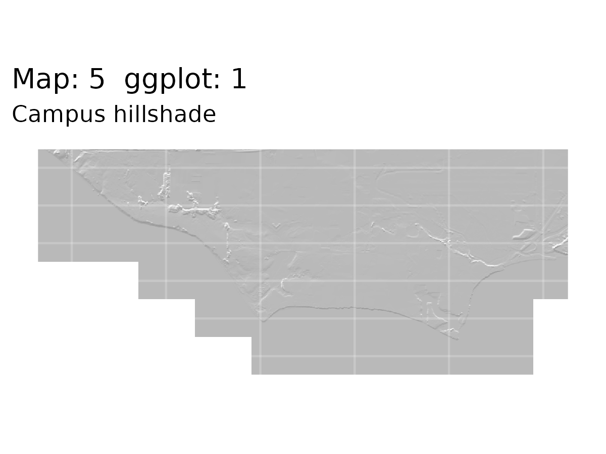
  ggtitle(gg_labelmaker(current_ggplot+1), subtitle = "Campus hillshade")

zoom_3_plot
ggsave("images/map5.1.png", width = 4, height = 3, plot = zoom_3_plot, bg = "white")

# ggplot the DEM
zoom_3_DEM_df <- as.data.frame(campus_DEM, xy=TRUE)
str(zoom_3_DEM_df)

zoom_3_plot <- ggplot() +
  geom_raster(data = zoom_3_DEM_df,
              aes(x=x, y=y, fill=greatercampusDEM_1_1)) +
  scale_fill_viridis_c(guide="none") +
  my_theme +
  coord_sf() +
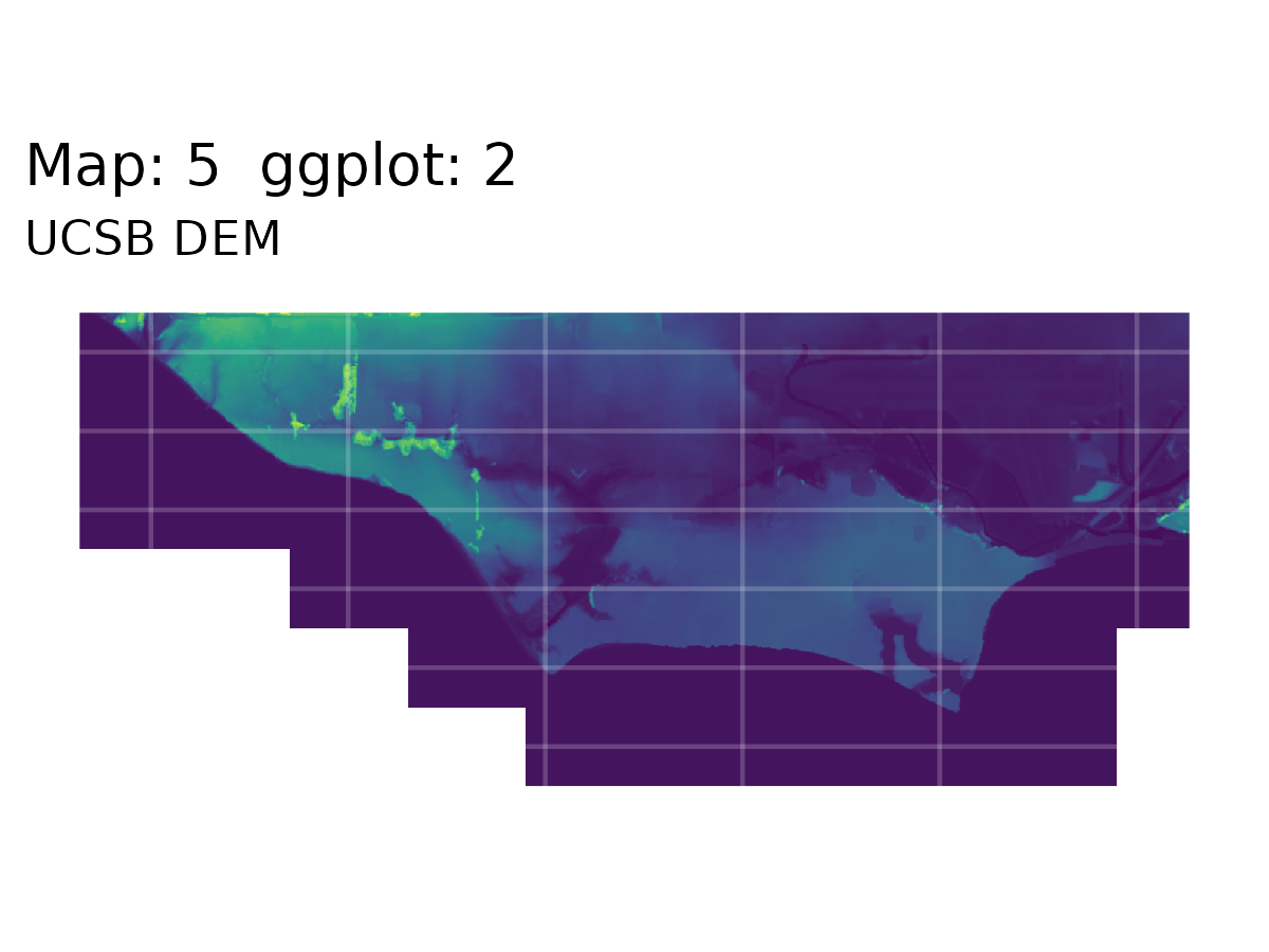
  ggtitle(gg_labelmaker(current_ggplot+1), subtitle = "UCSB DEM")

zoom_3_plot
ggsave("images/map5.2.png", width = 4, height = 3, plot = zoom_3_plot, bg = "white")

# now overlay
zoom_3_plot <- ggplot() +
  geom_raster(data = zoom_3_DEM_df,
              aes(x=x, y=y, fill=greatercampusDEM_1_1)) +
  scale_fill_viridis_c(guide = "none") +
  geom_raster(data = zoom_3_hillshade_df,
              aes(x=x, y=y, alpha=hillshade)) +
  scale_alpha(range = c(0.05, 0.5), guide="none") +
  my_theme +
  coord_sf() +
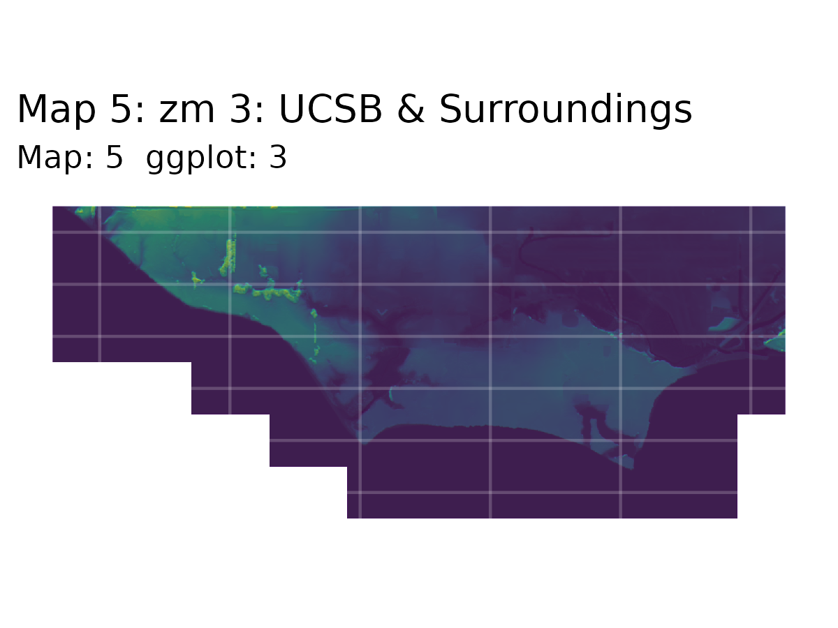
  ggtitle("Map 5: zm 3: UCSB & Surroundings", subtitle = gg_labelmaker(current_ggplot+1))

zoom_3_plot
ggsave("images/map5.3.png", width = 4, height = 3, plot = zoom_3_plot, bg = "white")

# back out of the shortened theme and use what works
zoom_3_plot <- ggplot() +
  geom_raster(data = zoom_3_DEM_df,
              aes(x=x, y=y, fill=greatercampusDEM_1_1)) +
  scale_fill_viridis_c(guide = "none") +
  geom_raster(data = zoom_3_hillshade_df,
              aes(x=x, y=y, alpha=hillshade)) +
  scale_alpha(range = c(0.05, 0.5), guide="none") +
  my_theme +
  coord_sf() +
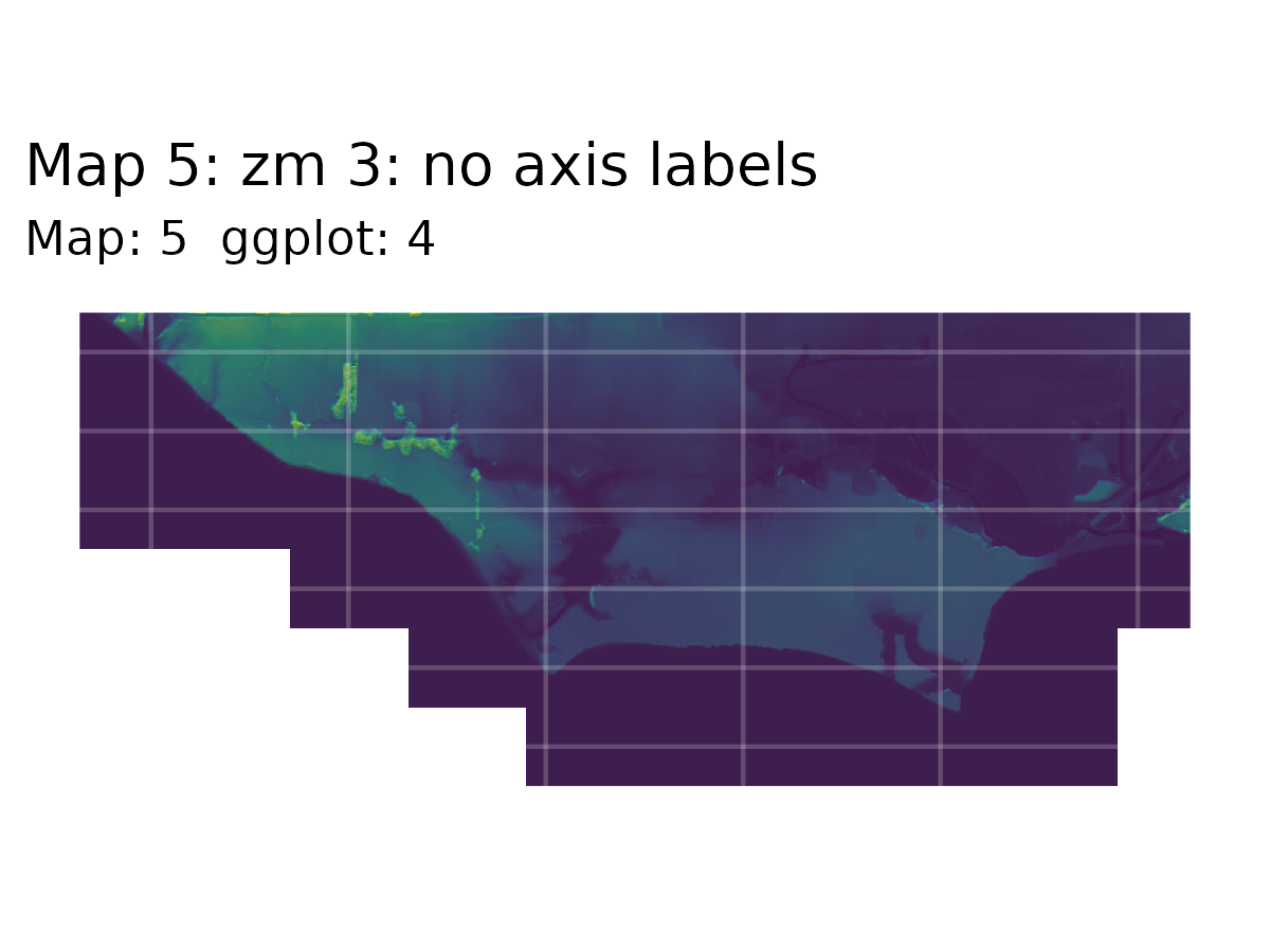
  ggtitle("Map 5: zm 3: no axis labels", subtitle = gg_labelmaker(current_ggplot+1))

zoom_3_plot
ggsave("images/map5.4.png", width = 4, height = 3, plot = zoom_3_plot, bg = "white")

# back out of the shortened theme and use what works
zoom_3_plot <- ggplot() +
  geom_raster(data = zoom_3_DEM_df,
              aes(x=x, y=y, fill=greatercampusDEM_1_1)) +
  scale_fill_viridis_c(guide = "none") +
  geom_raster(data = zoom_3_hillshade_df,
              aes(x=x, y=y, alpha=hillshade)) +
  scale_alpha(range = c(0.05, 0.5), guide="none") +
  my_theme +
  coord_sf() +
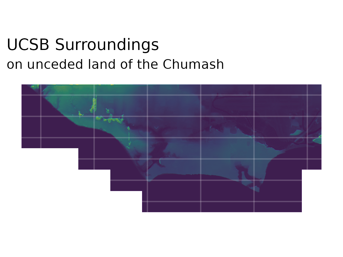
  ggtitle("UCSB Surroundings", subtitle = "on unceded land of the Chumash")

zoom_3_plot
ggsave("images/map5.5.png", width = 4, height = 3, plot = zoom_3_plot, bg = "white")


# zoom 3 needs water, bathymetry raster, buildings and bike paths
campus_bath <- rast("output_data/campus_bath_epsg2874.tif")
campus_bath_df <- as.data.frame(campus_bath, xy=TRUE) %>%
  rename(bathymetry = Bathymetry_2m_OffshoreCoalOilPoint)

# vector layers: buildings and bike paths
buildings <- st_read("source_data/campus_buildings/Campus_Buildings.shp")
iv_buildings <- st_read("source_data/iv_buildings/iv_buildings/CA_Structures_ExportFeatures.shp")
bikeways <- st_read("source_data/icm_bikes/bike_paths/bikelanescollapsedv8.shp")
ncos_trails <- st_read("source_data/ncos_trails/ncos_multiuse_trails.geojson")

camp_crs <- crs(campus_DEM)
buildings <- st_transform(buildings, camp_crs)
iv_buildings <- st_transform(iv_buildings, camp_crs)
bikeways <- st_transform(bikeways, camp_crs)
ncos_trails <- st_transform(ncos_trails, camp_crs)

# add bathymetry, hillshade, buildings and bike paths to the ggplot:
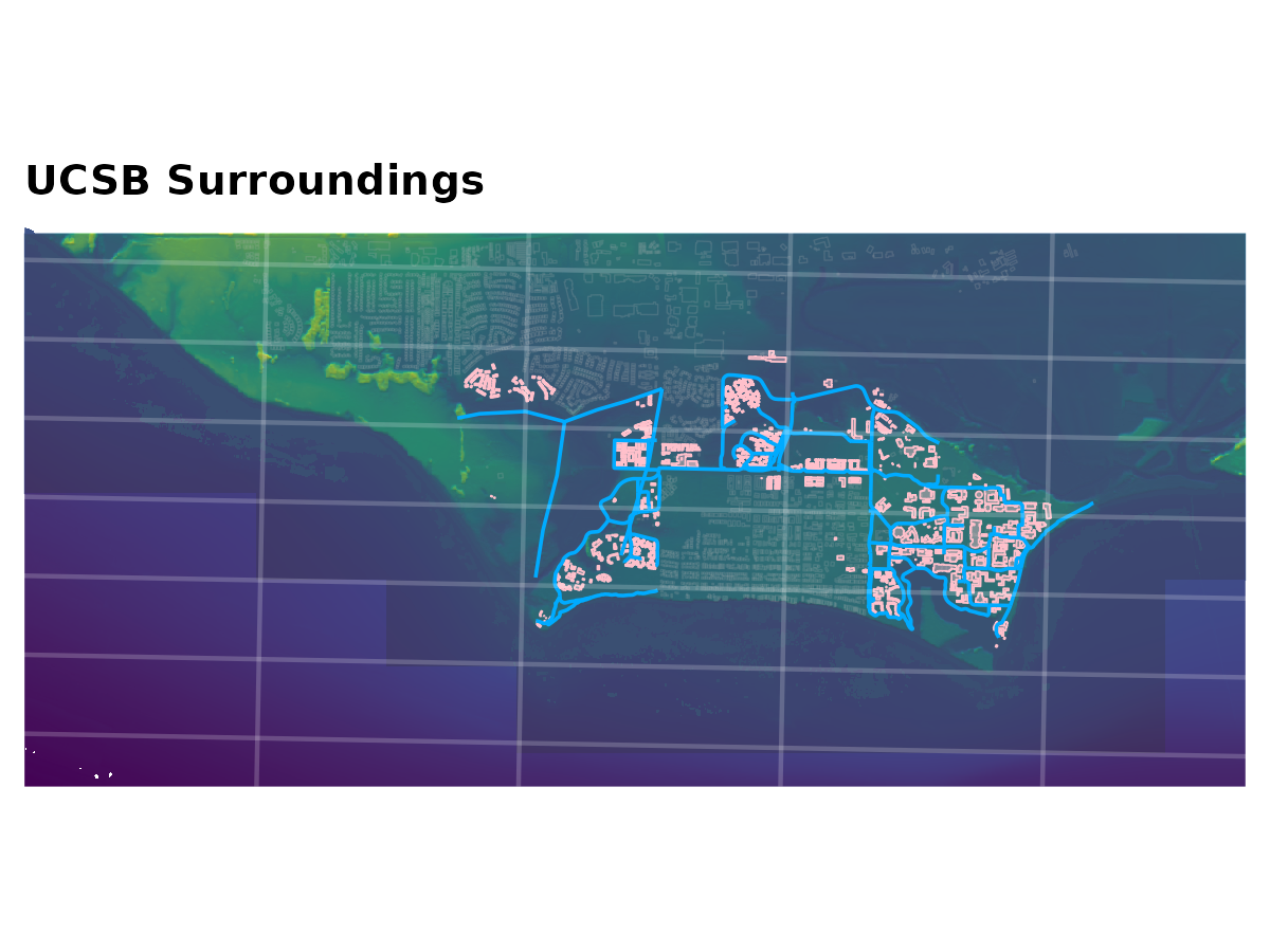
zoom_3_plot <- ggplot() +
  geom_raster(data = zoom_3_DEM_df,
              aes(x=x, y=y, fill=greatercampusDEM_1_1)) +
  geom_raster(data = campus_bath_df,
              aes(x=x, y=y, fill=bathymetry)) +
  scale_fill_viridis_c(na.value = "NA", guide = "none") +
  geom_raster(data = zoom_3_hillshade_df,
              aes(x=x, y=y, alpha=hillshade)) +
  scale_alpha(range = c(0.05, 0.4), guide="none") +
  geom_sf(data = iv_buildings, color = alpha("gray70", 0.2), fill = NA, linewidth = 0.15) +
  geom_sf(data = buildings, color = "pink", fill = alpha("pink", 0.4), linewidth = 0.2) +
  geom_sf(data = bikeways, color = "#00abff", linewidth = 0.4) +
  geom_sf(data = ncos_trails, color = "#00abff", linewidth = 0.4) +
  my_theme +
  coord_sf(expand = FALSE) +
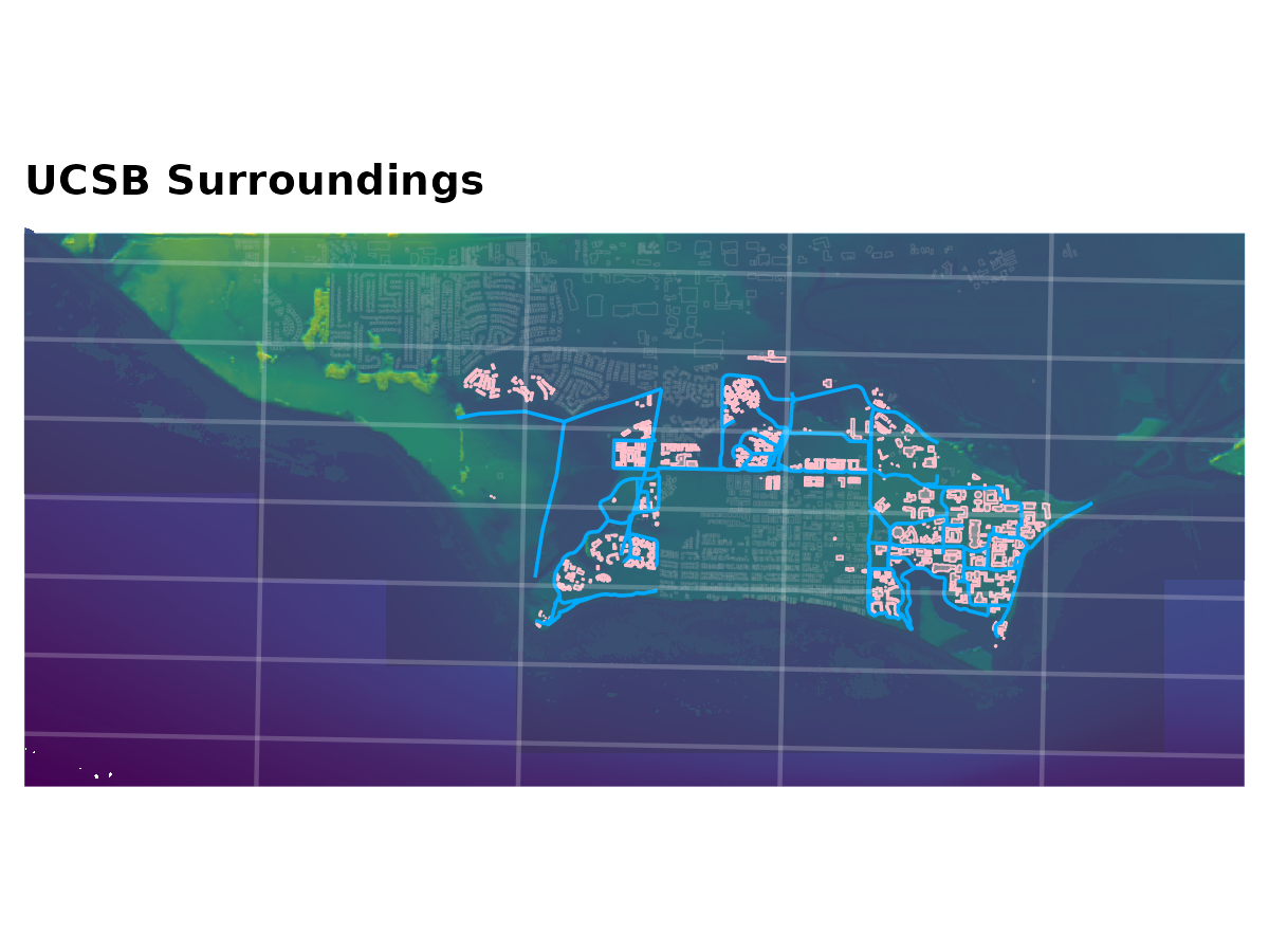
  ggtitle("UCSB Surroundings")

zoom_3_plot
ggsave("images/map5.6.png", width = 4, height = 3, plot = zoom_3_plot, bg = "white")

ggsave("images/map5.png", width = 4, height = 3, plot = zoom_3_plot, bg = "white")
ggsave("final_output/map_05.png", width = 4, height = 3, plot = zoom_3_plot, bg = "white")