---
title: "Map 8: Satellite Remote Sensing"
subtitle: "Multi-band PlanetScope satellite imagery and false-color composites"
---
## Rendered Map Plate
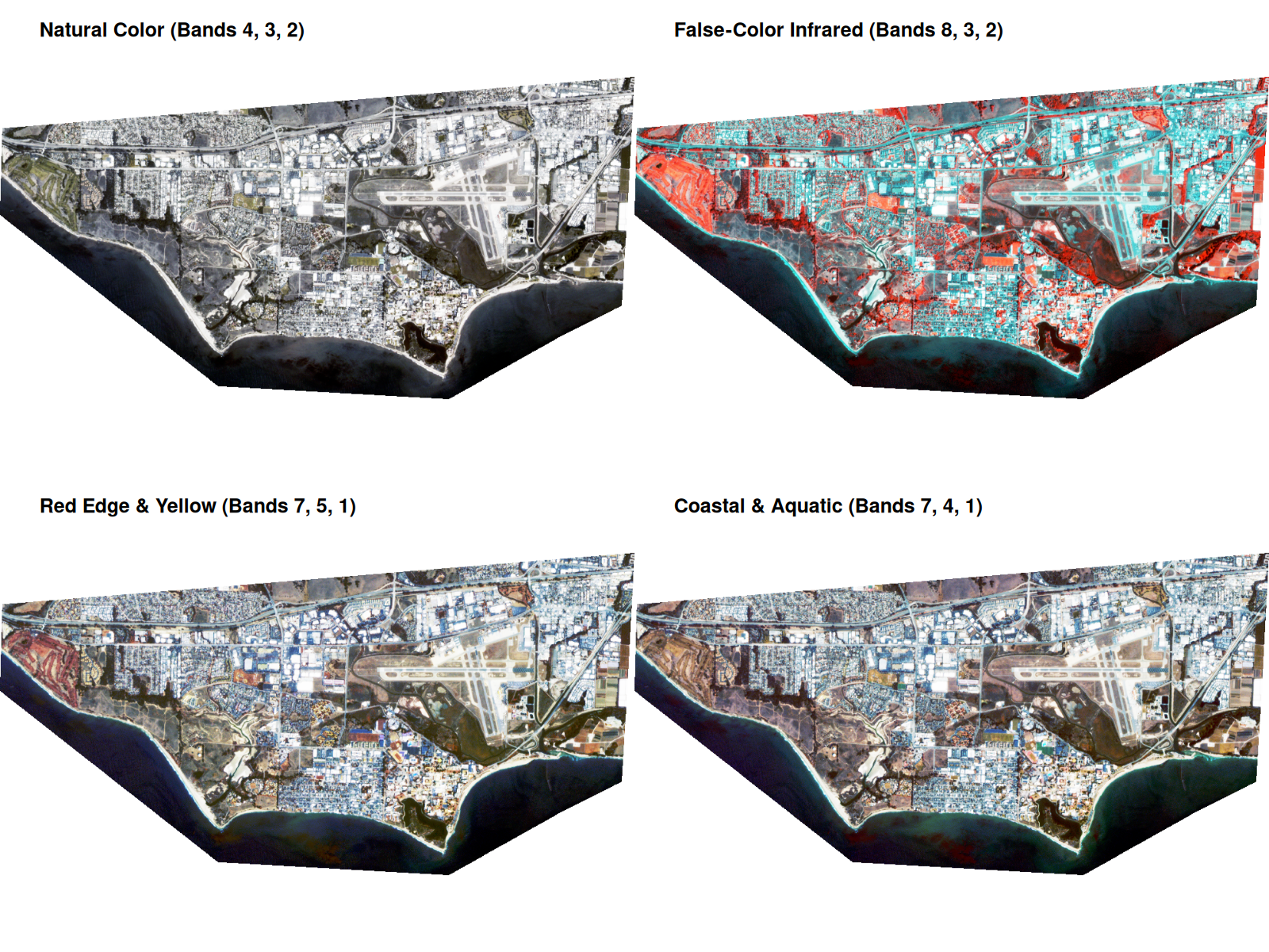{fig-alt="Map 8 PlanetScope Satellite Imagery" width="100%"}
---
## Technical Summary
* **Objective:** Explore multi-band raster manipulation using PlanetScope 4-band and 8-band high-resolution satellite scenes covering UCSB across multiple seasonal collections.
* **Key Packages:** `terra` (pure raster workflow)
* **Techniques Demonstrated:**
* Multi-band raster subsetting and indexing
* Natural color RGB compositing (`plotRGB` with linear stretch)
* False-color Infrared (CIR) compositing highlighting active photosynthetic vegetation
* Dynamic range scaling and histogram stretching
* **Output:** `final_output/map_08.png` (also archived at `final_output/map8.png`)
---
## Step-by-Step Cartographic Workflow & Intermediate Outputs
The script `scripts/map_08.r` is an all-`terra` workflow exploring multi-spectral remote sensing channels and false-color infrared composites.
### Step 1: Ingesting PlanetScope 8-Band Surface Reflectance
An 8-band PlanetScope AnalyticMS scene (`20230912_..._SR_8b_clip.tif`) is loaded into a `SpatRaster`. The scene features 3-meter pixel resolution and 8 spectral bands: Coastal Blue (1), Blue (2), Green I (3), Green II (4), Yellow (5), Red (6), Red Edge (7), and Near-Infrared / NIR (8).
```r
library(terra)

# Load 8-band surface reflectance cube
planet_scene <- rast("source_data/planet/planet/20232024_UCSB_campus_PlanetScope/PSScene/20230912_175450_00_2439_3B_AnalyticMS_SR_8b_clip.tif")

# Inspect raster metadata
dim(planet_scene) # Rows, columns, and 8 spectral bands
res(planet_scene) # ~3.0 meter ground sample distance
```
### Step 2: Dynamic Range Stretching (`stretch = "hist"` vs `"lin"`)
Raw 16-bit satellite reflectance values cluster in low radiometric values. Passing raw rasters to `plotRGB()` produces near-black outputs. The script applies dynamic range histogram equalization:
```r
# Testing stretch modes
plotRGB(planet_scene, stretch = "lin")
plotRGB(planet_scene, stretch = "hist")
```
### Step 3: Spectral Band Combinations & Quadrant Compositing
By mapping non-visible spectral wavelengths into standard red-green-blue display channels, different physical phenomena emerge:
1. **Natural Color (`r=4, g=3, b=2`):** Green, Blue, and Coastal Blue approximate true human vision.
2. **False-Color Infrared (`r=8, g=3, b=2`):** Maps Near-Infrared (Band 8) into the Red channel. Healthy chlorophyll strongly reflects NIR, causing athletic turf, Goleta Slough wetlands, and irrigated campus landscaping to glow bright crimson.
3. **Yellow-as-Green (`r=7, g=5, b=1`):** Highlights vegetation vigor using the Red Edge band (Band 7) and yellow reflectance (Band 5).
4. **Pretty High-Contrast (`r=7, g=4, b=1`):** Accentuates marine boundaries, sediment plumes, and urban structures using Red Edge and Coastal Blue.
```r
# Export 4-quadrant remote sensing comparison plate
png("final_output/map_08.png", width = 1200, height = 1200, res = 150)
par(mfrow = c(2, 2))

# 1. Natural Color
plotRGB(planet_scene, stretch = "hist", r = 4, g = 3, b = 2, main = "Natural Color (Bands 4, 3, 2)")

# 2. False-Color Infrared (CIR)
plotRGB(planet_scene, stretch = "hist", r = 8, g = 3, b = 2, main = "False-Color Infrared (Bands 8, 3, 2)")

# 3. Yellow = Green
plotRGB(planet_scene, stretch = "hist", r = 7, g = 5, b = 1, main = "Red Edge & Yellow (Bands 7, 5, 1)")

# 4. High-Contrast Composite
plotRGB(planet_scene, stretch = "hist", r = 7, g = 4, b = 1, main = "Coastal & Aquatic (Bands 7, 4, 1)")

dev.off()
```
{fig-alt="Map 8 Multi-Spectral Plate" width="70%"}
---
## Why Use Different Spectral Band Combinations?
Multispectral satellite sensors record electromagnetic radiation across discrete wavelength intervals, many of which extend beyond the range of human vision. Computer monitors and human visual systems are trichromatic—they render all imagery by combining three color channels: **Red**, **Green**, and **Blue** (RGB).
Because a multispectral sensor like PlanetScope SuperDove collects 8 distinct spectral bands, we cannot view all channels simultaneously in a single display. Instead, we create **spectral band composites** by assigning any three selected raster bands to the Red, Green, and Blue display channels of `plotRGB()`.
Different Earth surface materials—living vegetation, water, soil, asphalt, beach sand, and concrete—possess unique **spectral reflectance signatures**. Choosing specific band combinations enables analysts to exploit these signatures for specific environmental, biological, and urban mapping objectives.
### PlanetScope 8-Band Spectral Reference
The PlanetScope SuperDove (PSB.SD) instrument captures 8 surface reflectance bands across visible and near-infrared wavelengths:
| Band | Band Name | Wavelength Range | Key Biophysical Sensitivities & Remote Sensing Uses |
|:----:|:----------|:-----------------|:---------------------------------------------------|
| **1** | Coastal Blue | 431–452 nm | Water column penetration, coastal bathymetry, suspended sediment plumes, atmospheric aerosol scattering. |
| **2** | Blue | 465–515 nm | Water body mapping, soil vs. vegetation separation, atmospheric haze differentiation. |
| **3** | Green I | 513–549 nm | Chlorophyll reflectance peak in the green spectrum; water clarity and submerged aquatic features. |
| **4** | Green II | 547–583 nm | Broader green reflectance peak; assessment of healthy vegetation canopies and cultural green cover. |
| **5** | Yellow | 600–620 nm | Transition zone between green reflection and red absorption; sensitive to leaf senescence, yellowing (chlorosis), and crop maturity. |
| **6** | Red | 650–680 nm | Strong chlorophyll absorption band; provides maximum contrast between green vegetation and bare soil/built structures. |
| **7** | Red Edge | 697–713 nm | Steep spectral slope between visible absorption and NIR scattering; highly sensitive to pre-visual plant stress, canopy nitrogen, and moisture status. |
| **8** | Near-Infrared (NIR) | 845–885 nm | Strongly scattered by spongy mesophyll leaf cell structures; nearly 100% absorbed by liquid water; premier channel for biomass, vigor, and water boundaries. |
---
### Detailed Rationale for the Composites in Map 8
#### 1. Natural Color (`r=4, g=3, b=2`)
* **Wavelengths Used:** Green II (Band 4) $\rightarrow$ Red, Green I (Band 3) $\rightarrow$ Green, Blue (Band 2) $\rightarrow$ Blue.
* **Why You Might Want to Use It:**
* **Intuitive Baseline & Orientation:** Renders the scene as close as possible to human vision from an aircraft or spacecraft. Non-specialists can immediately identify familiar landmarks such as Storke Tower, Robertson Gym, Goleta Beach, and Isla Vista street grids without needing a spectral key.
* **Built Infrastructure & Beach Sand:** Urban features (parking lots, building footprints) and coastal sands reflect consistently across visible channels, making them easy to identify for baseline ground-truthing.
* **When NOT to Use It:** Natural color is relatively poor at distinguishing subtle plant stress, differentiating wetland vegetation types, or separating deep water bodies from dark shadows or fresh asphalt.
#### 2. False-Color Infrared / CIR (`r=8, g=3, b=2`)
* **Wavelengths Used:** Near-Infrared (Band 8) $\rightarrow$ Red, Green I (Band 3) $\rightarrow$ Green, Blue (Band 2) $\rightarrow$ Blue.
* **Why You Might Want to Use It:**
* **Photosynthetic Vigor & Biomass Density:** Healthy, chlorophyll-dense vegetation absorbs visible red light but strongly reflects NIR radiation (up to 50% reflectance) due to internal leaf cell structure. By routing Band 8 (NIR) to the Red display channel, actively transpiring vegetation pops in **vibrant crimson and magenta**. Heavily irrigated campus turf (Rec Cen sports fields, Storke Field, Harder Stadium) and lush eucalyptus groves glow bright red, while dry summer chaparral appears faded pink or brown.
* **Crisp Land–Water Interface:** Liquid water absorbs almost all NIR radiation. Consequently, water features like the Campus Lagoon, Goleta Slough channels, Devereux Slough, and the Pacific Ocean appear as **jet-black or deep inky-blue** voids. This produces sharp, unambiguous boundaries along coastlines, sand spits, and estuarine shorelines.
* **Urban Separation:** Concrete, asphalt roads, and bare soil reflect similarly in visible and NIR wavelengths, appearing in cool cyan, silver, or tan tones, neatly separating artificial hardscape from living green spaces.
#### 3. Yellow-as-Green / Red Edge & Yellow (`r=7, g=5, b=1`)
* **Wavelengths Used:** Red Edge (Band 7) $\rightarrow$ Red, Yellow (Band 5) $\rightarrow$ Green, Coastal Blue (Band 1) $\rightarrow$ Blue.
* **Why You Might Want to Use It:**
* **Pre-Visual Plant Stress Detection:** The "Red Edge" (697–713 nm) is the steep transition zone between chlorophyll absorption in the red and cell scattering in the NIR. Stressed vegetation (experiencing drought, disease, or nitrogen deficiency) shows a measurable shift in the red-edge slope days to weeks before visible wilting or yellowing occurs.
* **Canopy Chemistry & Senescence:** Band 5 (Yellow) directly measures carotenoid pigment concentrations and drying foliage. Pairing Red Edge with Yellow distinguishes between actively growing canopies, senescent vegetation, and dying invasive grasses across the campus bluffs and Goleta Slough.
* **Habitat Classification:** Provides superior contrast for discriminating between native coastal scrub, non-native grasses, and salt marsh species that look uniformly green or brown in true-color imagery.
#### 4. High-Contrast Coastal / Aquatic Composite (`r=7, g=4, b=1`)
* **Wavelengths Used:** Red Edge (Band 7) $\rightarrow$ Red, Green II (Band 4) $\rightarrow$ Green, Coastal Blue (Band 1) $\rightarrow$ Blue.
* **Why You Might Want to Use It:**
* **Nearshore Oceanographic Dynamics & Sediment Plumes:** Band 1 (Coastal Blue) has the shortest wavelength and deepest water penetration of any satellite band. It scatters strongly off suspended sediments, terrestrial runoff, and surf breaks. Combining it with Green and Red Edge accentuates sediment plumes off Goleta Pier and Campus Point.
* **Surf Zone & Kelp Forest Mapping:** Accentuates the boundary between offshore open ocean water, breaking surf along the campus point, and nearshore giant kelp (*Macrocystis pyrifera*) canopies floating on the sea surface.
* **Maximum Radiometric Dynamic Range:** By spanning shortwave coastal blue (431 nm) to red edge (713 nm), this composite maximizes tonal separation across the marine-terrestrial transition zone of the UCSB peninsula.
---
### Campus Application Matrix: Which Band Combination Should You Choose?
| Monitoring or Research Task | Recommended Composite | Key Bands Used | What to Look For on Campus |
|:----------------------------|:----------------------|:---------------|:---------------------------|
| **Campus Irrigation & Turf Audit** | False-Color Infrared (CIR) | Bands 8, 3, 2 | Bright crimson shows irrigated lawns (Rec Cen, Storke Field); pale pink indicates drought-stressed or dormant lawns. |
| **Wetland & Shoreline Boundary Mapping** | False-Color Infrared (CIR) | Bands 8, 3, 2 | Ink-black water creates high-contrast edges along Campus Lagoon and Goleta Slough tidal channels. |
| **Early Plant Stress & Canopy Health** | Red Edge & Yellow | Bands 7, 5, 1 | Tonal shifts in the Red Edge reveal water stress in campus trees and bluff vegetation before visible browning. |
| **Nearshore Sediments & Kelp Beds** | Coastal High-Contrast | Bands 7, 4, 1 | Coastal Blue reveals suspended sediment plumes off Campus Point and surf zone breaks; Red Edge reveals floating kelp. |
| **Campus Master Planning & Infrastructure** | Natural Color | Bands 4, 3, 2 | Familiar, photorealistic view for building footprints, parking structures, and walkway orientation. |
---
## Full R Script (`scripts/map_08.r`)
```{r}
#| eval: false
#| code: !expr readLines("../scripts/map_08.r")
```

