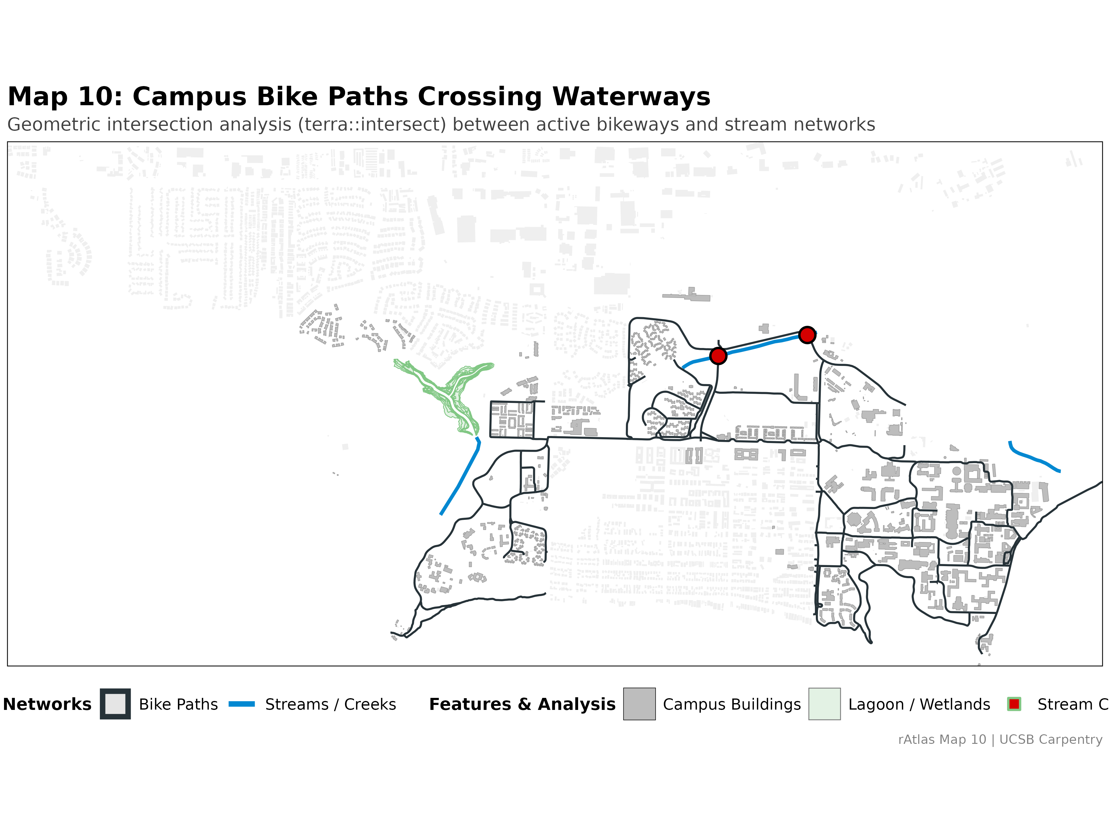
# Map 10: Vector Intersection Analysis - Bike Paths Crossing Creeks
library(terra)
library(tidyverse)
library(tidyterra)
library(sf)

# Clean the environment and hidden objects
rm(list = ls())

# Set map number
current_sheet <- 10
# Set ggplot counter
current_ggplot <- 0

gg_labelmaker <- function(plot_num) {
  gg_title <- c("Map:", current_sheet, " ggplot:", plot_num)
  plot_text <- paste(gg_title, collapse = " ")
  print(plot_text)
  current_ggplot <<- plot_num
  return(plot_text)
}

# Ensure output directories exist
dir.create("images", showWarnings = FALSE)
dir.create("final_output", showWarnings = FALSE)
dir.create("output_data", showWarnings = FALSE)

# ---------- 1. Read Vector Layers ----------
bike_paths <- vect("source_data/icm_bikes/bike_paths/bikelanescollapsedv8.shp")
creeks <- vect("source_data/california_streams/streams_crop.shp")
buildings <- vect("source_data/campus_buildings/Campus_Buildings.shp")
iv_bldg <- vect("source_data/iv_buildings/iv_buildings/CA_Structures_ExportFeatures.shp")
habitat <- vect("source_data/NCOS_Shorebird_Foraging_Habitat/NCOS_Shorebird_Foraging_Habitat.shp")

# ---------- 2. Align to Common CRS ----------
target_crs <- crs(bike_paths)
creeks <- project(creeks, target_crs)
buildings <- project(buildings, target_crs)
iv_bldg <- project(iv_bldg, target_crs)
habitat <- project(habitat, target_crs)

# ---------- 3. Perform Intersection Analysis ----------
# Compute geometric intersection between stream lines and bike path networks
creek_bike_pts <- terra::intersect(creeks, bike_paths)
creek_bike_pts_disagg <- disagg(creek_bike_pts)

cat("Intersection analysis complete: found", length(creek_bike_pts_disagg), "crossing points.\n")

# ---------- 4. Export Resulting Vector Points ----------
out_file <- "output_data/creek_bike_intersections.shp"
writeVector(creek_bike_pts, out_file, overwrite = TRUE)
cat("Exported crossing points to:", out_file, "\n")

# ---------- 5. Construct Cartographic Layout ----------
map10_plot <- ggplot() +
  # Habitat and context polygons
  geom_spatvector(data = habitat, aes(fill = "Lagoon / Wetlands"), color = "#81C784", linewidth = 0.3, alpha = 0.5) +
  geom_spatvector(data = iv_bldg, fill = "#E0E0E080", color = NA) +
  geom_spatvector(data = buildings, aes(fill = "Campus Buildings"), color = "#9E9E9E", linewidth = 0.2) +
  # Linear networks
  geom_spatvector(data = creeks, aes(color = "Streams / Creeks"), linewidth = 1.3) +
  geom_spatvector(data = bike_paths, aes(color = "Bike Paths"), linewidth = 0.75) +
  # Highlighted intersection points
  geom_spatvector(data = creek_bike_pts_disagg, aes(fill = "Stream Crossings"), shape = 21, size = 5, color = "black", stroke = 1.3) +
  # Scales & aesthetics
  scale_color_manual(
    name = "Linear Networks",
    values = c("Streams / Creeks" = "#0288D1", "Bike Paths" = "#263238"),
    guide = guide_legend(override.aes = list(linewidth = 2), order = 1)
  ) +
  scale_fill_manual(
    name = "Features & Analysis",
    values = c("Stream Crossings" = "#D50000", "Campus Buildings" = "#BDBDBD", "Lagoon / Wetlands" = "#C8E6C9"),
    guide = guide_legend(override.aes = list(shape = c(21, 22, 22), size = c(5, 4, 4), color = c("black", "#757575", "#81C784")), order = 2)
  ) +
  theme_minimal() +
  theme(
    plot.title = element_text(face = "bold", size = 20, hjust = 0.5),
    plot.subtitle = element_text(size = 14, hjust = 0.5, color = "gray25"),
    plot.caption = element_text(size = 10, color = "gray50"),
    axis.title = element_blank(),
    axis.text = element_blank(),
    axis.ticks = element_blank(),
    panel.grid = element_blank(),
    panel.border = element_rect(color = "black", fill = NA, linewidth = 0.6),
    legend.position = "bottom",
    legend.box = "horizontal",
    legend.title = element_text(face = "bold", size = 13),
    legend.text = element_text(size = 12),
    legend.key.size = unit(0.9, "cm"),
    legend.spacing.x = unit(0.5, "cm")
  ) +
  coord_sf(expand = FALSE) +
  labs(
    title = "Map 10: Campus Bike Paths Crossing Waterways",
    subtitle = "Geometric intersection analysis (terra::intersect) between active bikeways and stream networks",
    caption = "rAtlas Map 10 | UCSB Carpentry"
  )

# ---------- 6. Save Publication Outputs ----------
ggsave("images/map10.png", plot = map10_plot, width = 12, height = 9, dpi = 300, bg = "white")
ggsave("final_output/map_10.png", plot = map10_plot, width = 12, height = 9, dpi = 300, bg = "white")

cat("Map 10 saved to:\n")
cat(" - images/map10.png\n")
cat(" - final_output/map_10.png\n")